Practical session on `xarray`¶

Instructions¶

Load the python-training/misc/data/mesh_mask_eORCA1_v2.2.nc file using open_dataset.

Extract the surface (z=0) and first time step (t=0) using isel

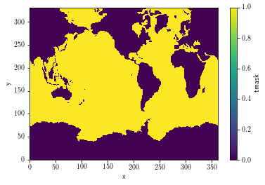
Plot the land-sea mask (tmask) variable.

Compute the cell surface (e1t x e2t)

Load the python-training/misc/data/surface_thato.nc file using open_dataset.

Extract the SST (thetao variable) at the surface (olevel=0)

Compute and display the time-average SST

Compute the mean SST over years 1958-1962

Compute the mean over years 2014-2018

Plot the SST difference between 2018-2014 and 1958-1962

Compute the SST global mean time-series (weight by cell surface $e1t \times e2t$)

Remove the monthly clim from the time-series using groupy on time_counter.month

Compute the rolling mean of the time-series, using a 3-year window. Plot the raw and smoothed anomalies

Corrections¶

Load the python-training/misc/data/mesh_mask_eORCA1_v2.2.nc file using open_dataset.

Extract the surface (z=0) and first time step (t=0) using isel

Plot the land-sea mask (tmask) variable.

tmask = mesh['tmask']
tmask.plot()

<matplotlib.collections.QuadMesh at 0x7f3ce4b62e90>

Compute the cell surface (e1t x e2t)

surface = mesh['e1t'] * mesh['e2t']
surface

<xarray.DataArray (y: 332, x: 362)>
array([[1.60000000e+01, 1.60000000e+01, 1.60000000e+01, ...,
        1.60000000e+01, 1.60000000e+01, 1.60000000e+01],
       [1.60000000e+01, 1.60000000e+01, 1.60000000e+01, ...,
        1.60000000e+01, 1.60000000e+01, 1.60000000e+01],
       [1.60000000e+01, 1.60000000e+01, 1.60000000e+01, ...,
        1.60000000e+01, 1.60000000e+01, 1.60000000e+01],
       ...,
       [4.96784478e+07, 4.96784478e+07, 1.68195300e+08, ...,
        1.68195300e+08, 4.96784478e+07, 4.96784478e+07],
       [3.18035791e+07, 3.18035791e+07, 1.55003643e+08, ...,
        1.55003643e+08, 3.18035791e+07, 3.18035791e+07],
       [3.18035791e+07, 3.18035791e+07, 1.55003643e+08, ...,
        1.55003643e+08, 3.18035791e+07, 3.18035791e+07]])
Dimensions without coordinates: y, x

Here the output DatarArray has no name. You can give him one as follows:

surface.name = 'surface'
surface

<xarray.DataArray 'surface' (y: 332, x: 362)>
array([[1.60000000e+01, 1.60000000e+01, 1.60000000e+01, ...,
        1.60000000e+01, 1.60000000e+01, 1.60000000e+01],
       [1.60000000e+01, 1.60000000e+01, 1.60000000e+01, ...,
        1.60000000e+01, 1.60000000e+01, 1.60000000e+01],
       [1.60000000e+01, 1.60000000e+01, 1.60000000e+01, ...,
        1.60000000e+01, 1.60000000e+01, 1.60000000e+01],
       ...,
       [4.96784478e+07, 4.96784478e+07, 1.68195300e+08, ...,
        1.68195300e+08, 4.96784478e+07, 4.96784478e+07],
       [3.18035791e+07, 3.18035791e+07, 1.55003643e+08, ...,
        1.55003643e+08, 3.18035791e+07, 3.18035791e+07],
       [3.18035791e+07, 3.18035791e+07, 1.55003643e+08, ...,
        1.55003643e+08, 3.18035791e+07, 3.18035791e+07]])
Dimensions without coordinates: y, x

Load the python-training/misc/data/surface_thato.nc file using open_dataset.

Extract the SST (thetao variable) at the surface (olevel=0)

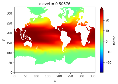
Compute and display the time-average SST

import matplotlib.pyplot as plt
plt.rcParams['text.usetex'] = False

theta_mean = thetao.mean(dim='time_counter')
theta_mean.plot(robust=True, cmap=plt.cm.jet)

<matplotlib.collections.QuadMesh at 0x7f3ce366be90>

Compute the mean SST over years 1958-1962

sst_early = thetao.sel(time_counter=slice('1958-01-01', '1962-12-31')).mean(dim='time_counter')
sst_early

<xarray.DataArray 'thetao' (y: 332, x: 362)>
array([[nan, nan, nan, ..., nan, nan, nan],
       [nan, nan, nan, ..., nan, nan, nan],
       [nan, nan, nan, ..., nan, nan, nan],
       ...,
       [nan, nan, nan, ..., nan, nan, nan],
       [nan, nan, nan, ..., nan, nan, nan],
       [nan, nan, nan, ..., nan, nan, nan]], dtype=float32)
Coordinates:
    nav_lat  (y, x) float32 ...
    nav_lon  (y, x) float32 ...
    olevel   float32 0.5058
Dimensions without coordinates: y, x

Compute the mean over years 2014-2018

sst_late = thetao.sel(time_counter=slice('2014-01-01', '2018-12-31')).mean(dim='time_counter')
sst_late

<xarray.DataArray 'thetao' (y: 332, x: 362)>
array([[nan, nan, nan, ..., nan, nan, nan],
       [nan, nan, nan, ..., nan, nan, nan],
       [nan, nan, nan, ..., nan, nan, nan],
       ...,
       [nan, nan, nan, ..., nan, nan, nan],
       [nan, nan, nan, ..., nan, nan, nan],
       [nan, nan, nan, ..., nan, nan, nan]], dtype=float32)
Coordinates:
    nav_lat  (y, x) float32 ...
    nav_lon  (y, x) float32 ...
    olevel   float32 0.5058
Dimensions without coordinates: y, x

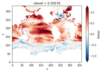
Plot the SST difference between 2014-2018 and 1958-1962

(sst_late - sst_early).plot(robust=True)

<matplotlib.collections.QuadMesh at 0x7f3ce35de790>

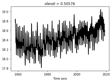
Compute the SST global mean time-series (weight by cell surface $e1t \times e2t$)

A first possibility would be to compute it using sum:

ts1 = (thetao * surface * tmask).sum(dim=['x', 'y']) / ((surface * tmask).sum(dim=['x', 'y']))
ts1.plot()

[<matplotlib.lines.Line2D at 0x7f3ce34d2ad0>]

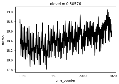
Another solution would be to use the xarray.weight method:

theta_weighted = thetao.weighted(surface * tmask)
ts2 = theta_weighted.mean(dim=['x', 'y'])
ts2.plot()

[<matplotlib.lines.Line2D at 0x7f3ce3460bd0>]

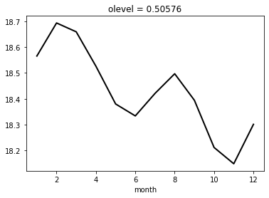
Remove the monthly clim from the time-series using groupy on time_counter.month

clim = ts1.groupby('time_counter.month').mean(dim='time_counter')
clim.plot()

[<matplotlib.lines.Line2D at 0x7f3ce15c4d10>]

anom = ts1.groupby('time_counter.month') - clim
anom.plot()

[<matplotlib.lines.Line2D at 0x7f3ce1553350>]

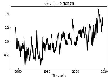
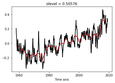
Compute the rolling mean of the time-series, using a 3-year window. Plot the raw and smoothed anomalies

anom.plot(label='raw')
tsroll.plot(label='smoothed')

[<matplotlib.lines.Line2D at 0x7f3ce14dad50>]

Introduction to Python

Practical session on xarray¶

Instructions¶

Corrections¶

Practical session on `xarray`¶