.ipynb .pdf

repository open issue

Binder

Contents

NetCDF

A very efficient way to read, analyze and write NetCDF files is to use the xarray Python library, which can be viewed as a ND counterpart of the pandas.

Reading NetCDF

Reading single file

Reading NetCDF files is dones by using the xarray.open_dataset method, which returns a xarray.Dataset object.

import xarray as xr
import numpy as np

data = xr.open_dataset('data/UV500storm.nc')
data

<xarray.Dataset>
Dimensions:   (lat: 33, lon: 36, timestep: 1)
Coordinates:
  * lat       (lat) float32 20.0 21.25 22.5 23.75 25.0 ... 56.25 57.5 58.75 60.0
  * lon       (lon) float32 -140.0 -137.5 -135.0 -132.5 ... -57.5 -55.0 -52.5
  * timestep  (timestep) int32 372
Data variables:
    reftime   |S20 b'1996 01 05 00:00'
    v         (timestep, lat, lon) float32 nan nan nan nan ... 54.32 49.82 44.32
    u         (timestep, lat, lon) float32 nan nan nan nan ... 7.713 8.213 9.713
Attributes:
    history:  Thu Jul 21 16:12:12 2016: ncks -A U500storm.nc V500storm.nc\nTh...
    NCO:      4.4.2

Reading multiple files

Often, a variable is stored in multiple NetCDF files (one file per year for instance). The xarray.open_mfdataset allows to open all the files at one and to concatenate them along record dimension (UNLIMITED dimension, which is usually time) and spatial dimensions.

Below, the four ISAS13 files are opened at once and are automatically concanated along the record dimension, hence leading to a dataset with 4 time steps.

data = xr.open_mfdataset("data/*ISAS*nc", combine='by_coords')
data

<xarray.Dataset>
Dimensions:  (time: 4, depth: 152)
Coordinates:
  * depth    (depth) float32 0.0 3.0 5.0 10.0 ... 1.96e+03 1.98e+03 2e+03
  * time     (time) datetime64[ns] 2012-01-15 2012-02-15 2012-03-15 2012-04-15
Data variables:
    TEMP     (time, depth) float32 dask.array<chunksize=(1, 152), meta=np.ndarray>
Attributes:
    script:   extract_prof.py
    history:  Thu Jul 14 11:32:10 2016: ncks -O -3 ISAS13_20120115_fld_TEMP.n...
    NCO:      "4.5.5"

Furthermore, complex models are often paralellized using the Message Passing Interface (MPI), in which each processor manages a subdomain. If each processor saves output in its sub-region, there will be as many output files as there are processors. xarray allows to reconstruct the global file by concatenating the subregional files according to their coordinates.

Warning! This actually works only if the decomposition into subregions is regular, and if subfiles contain coordinates

data = xr.open_mfdataset("data/GYRE_OOPE*", combine='by_coords', engine='netcdf4')
data['OOPE']

<xarray.DataArray 'OOPE' (time: 10, y: 22, x: 32, community: 3, weight: 100)>
dask.array<concatenate, shape=(10, 22, 32, 3, 100), dtype=float32, chunksize=(10, 11, 16, 3, 100), chunktype=numpy.ndarray>
Coordinates:
  * x        (x) int64 0 1 2 3 4 5 6 7 8 9 10 ... 22 23 24 25 26 27 28 29 30 31
  * y        (y) int64 0 1 2 3 4 5 6 7 8 9 10 11 12 13 14 15 16 17 18 19 20 21
Dimensions without coordinates: time, community, weight

In the 2 previous examples, chunksize variable attribute appeared. This is due to the fact that opening multiple datasets automatically generates dask arrays, which are ready for parallel computing. These are discussed in a specific section

Accessing dimensions, variables, attributes

data = xr.open_dataset("data/UV500storm.nc")
data

<xarray.Dataset>
Dimensions:   (lat: 33, lon: 36, timestep: 1)
Coordinates:
  * lat       (lat) float32 20.0 21.25 22.5 23.75 25.0 ... 56.25 57.5 58.75 60.0
  * lon       (lon) float32 -140.0 -137.5 -135.0 -132.5 ... -57.5 -55.0 -52.5
  * timestep  (timestep) int32 372
Data variables:
    reftime   |S20 b'1996 01 05 00:00'
    v         (timestep, lat, lon) float32 nan nan nan nan ... 54.32 49.82 44.32
    u         (timestep, lat, lon) float32 nan nan nan nan ... 7.713 8.213 9.713
Attributes:
    history:  Thu Jul 21 16:12:12 2016: ncks -A U500storm.nc V500storm.nc\nTh...
    NCO:      4.4.2

Dimensions

Recovering dimensions is dony by accessing the dims attribute of the dataset, which returns a dictionary, the keys of which are the dataset dimension names and the values are the number of elements along the dimension.

data.dims

Frozen({'lat': 33, 'lon': 36, 'timestep': 1})

data.dims['lat']

33

Variables

Variables can be accessed by using the data_vars attribute, which returns a dictionary, the keys of which are the dataset variable names.

data.data_vars

Data variables:
    reftime  |S20 b'1996 01 05 00:00'
    v        (timestep, lat, lon) float32 nan nan nan nan ... 54.32 49.82 44.32
    u        (timestep, lat, lon) float32 nan nan nan nan ... 7.713 8.213 9.713

data.data_vars['u']

<xarray.DataArray 'u' (timestep: 1, lat: 33, lon: 36)>
array([[[      nan,       nan, ...,       nan,       nan],
        [      nan,       nan, ...,       nan,       nan],
        ...,
        [ 0.213205, -0.036795, ..., 10.463205, 10.463205],
        [-2.036795, -1.536795, ...,  8.213205,  9.713205]]], dtype=float32)
Coordinates:
  * lat       (lat) float32 20.0 21.25 22.5 23.75 25.0 ... 56.25 57.5 58.75 60.0
  * lon       (lon) float32 -140.0 -137.5 -135.0 -132.5 ... -57.5 -55.0 -52.5
  * timestep  (timestep) int32 372

Note that data variables can also be accessed by using variable name as the key to the dataset object, as follows:

data['v']

<xarray.DataArray 'v' (timestep: 1, lat: 33, lon: 36)>
array([[[      nan,       nan, ...,       nan,       nan],
        [      nan,       nan, ...,       nan,       nan],
        ...,
        [-7.183777, -8.183777, ..., 48.816223, 42.316223],
        [-7.683777, -9.683777, ..., 49.816223, 44.316223]]], dtype=float32)
Coordinates:
  * lat       (lat) float32 20.0 21.25 22.5 23.75 25.0 ... 56.25 57.5 58.75 60.0
  * lon       (lon) float32 -140.0 -137.5 -135.0 -132.5 ... -57.5 -55.0 -52.5
  * timestep  (timestep) int32 372

Note that variables are returned as xarray.DataArray.

To recover the variable as a numpy array, the values attribute can be used. In this case, missing values are set to NaN.

v = data['v']
v = v.values
v

array([[[       nan,        nan,        nan, ...,        nan,
                nan,        nan],
        [       nan,        nan,        nan, ...,        nan,
                nan,        nan],
        [       nan,        nan,        nan, ...,        nan,
                nan,        nan],
        ...,
        [ -7.183777,  -7.683777,  -8.183777, ...,  53.316223,
          47.816223,  40.816223],
        [ -7.183777,  -8.183777,  -9.183777, ...,  53.816223,
          48.816223,  42.316223],
        [ -7.683777,  -9.683777, -11.683777, ...,  54.316223,
          49.816223,  44.316223]]], dtype=float32)

In order to obtain a masked array instead, use the to_masked_array() method:

v = data['v']
v = v.to_masked_array()
v

masked_array(
  data=[[[--, --, --, ..., --, --, --],
         [--, --, --, ..., --, --, --],
         [--, --, --, ..., --, --, --],
         ...,
         [-7.18377685546875, -7.68377685546875, -8.18377685546875, ...,
          53.31622314453125, 47.81622314453125, 40.81622314453125],
         [-7.18377685546875, -8.18377685546875, -9.18377685546875, ...,
          53.81622314453125, 48.81622314453125, 42.31622314453125],
         [-7.68377685546875, -9.68377685546875, -11.68377685546875, ...,
          54.31622314453125, 49.81622314453125, 44.31622314453125]]],
  mask=[[[ True,  True,  True, ...,  True,  True,  True],
         [ True,  True,  True, ...,  True,  True,  True],
         [ True,  True,  True, ...,  True,  True,  True],
         ...,
         [False, False, False, ..., False, False, False],
         [False, False, False, ..., False, False, False],
         [False, False, False, ..., False, False, False]]],
  fill_value=1e+20,
  dtype=float32)

Time management

By default, the time variable is detected by xarray by using the NetCDF attributes, and is converted into a human time. This is done by xarray by using the cftime module

data = xr.open_mfdataset("data/*ISAS*", combine='by_coords')
data['time']

<xarray.DataArray 'time' (time: 4)>
array(['2012-01-15T00:00:00.000000000', '2012-02-15T00:00:00.000000000',
       '2012-03-15T00:00:00.000000000', '2012-04-15T00:00:00.000000000'],
      dtype='datetime64[ns]')
Coordinates:
  * time     (time) datetime64[ns] 2012-01-15 2012-02-15 2012-03-15 2012-04-15

Then, the user can access the year, month, day, hour, minute, second, microsecond, nanosecond, date, time, dayofyear, weekofyear, dayofweek, quarter as follows:

data['time.year']

<xarray.DataArray 'year' (time: 4)>
array([2012, 2012, 2012, 2012])
Coordinates:
  * time     (time) datetime64[ns] 2012-01-15 2012-02-15 2012-03-15 2012-04-15

data['time.month']

<xarray.DataArray 'month' (time: 4)>
array([1, 2, 3, 4])
Coordinates:
  * time     (time) datetime64[ns] 2012-01-15 2012-02-15 2012-03-15 2012-04-15

data['time.day']

<xarray.DataArray 'day' (time: 4)>
array([15, 15, 15, 15])
Coordinates:
  * time     (time) datetime64[ns] 2012-01-15 2012-02-15 2012-03-15 2012-04-15

data['time.dayofyear']

<xarray.DataArray 'dayofyear' (time: 4)>
array([ 15,  46,  75, 106])
Coordinates:
  * time     (time) datetime64[ns] 2012-01-15 2012-02-15 2012-03-15 2012-04-15

Warning Replace time by the name of your time variable (time_counter in NEMO for instance)

If the user does not want xarray to convert time into a human date, set the decode_times argument to False.

data = xr.open_mfdataset("data/*ISAS*", combine='by_coords', decode_times=False)
data['time']

<xarray.DataArray 'time' (time: 4)>
array([22659., 22690., 22719., 22750.])
Coordinates:
  * time     (time) float64 2.266e+04 2.269e+04 2.272e+04 2.275e+04
Attributes:
    units:    days since 1950-01-01T00:00:00Z

In this case, years, months, etc. cannot be extracted

Attributes

To get variable attributes, use the attrs attribute, which exists for xarray.Dataset (global attributes) and xarray.DataArray objects (variable’s attributes). It returns a dictionary containing the attribute names and values.

data.attrs

{'script': 'extract_prof.py',
 'history': 'Thu Jul 14 11:32:10 2016: ncks -O -3 ISAS13_20120115_fld_TEMP.nc ISAS13_20120115_fld_TEMP.nc',
 'NCO': '"4.5.5"'}

data.attrs['NCO']

'"4.5.5"'

time = data['time']
time.attrs

{'units': 'days since 1950-01-01T00:00:00Z'}

time.attrs['units']

'days since 1950-01-01T00:00:00Z'

Indexing

As in pandas, there is 2 ways to extract part of a dataset. Let’s consider the ISAS dataset, which contains 152 vertical levels unevenly from 0 to 2000m.

data = xr.open_mfdataset('data/*ISAS*', combine='by_coords')
data

<xarray.Dataset>
Dimensions:  (time: 4, depth: 152)
Coordinates:
  * depth    (depth) float32 0.0 3.0 5.0 10.0 ... 1.96e+03 1.98e+03 2e+03
  * time     (time) datetime64[ns] 2012-01-15 2012-02-15 2012-03-15 2012-04-15
Data variables:
    TEMP     (time, depth) float32 dask.array<chunksize=(1, 152), meta=np.ndarray>
Attributes:
    script:   extract_prof.py
    history:  Thu Jul 14 11:32:10 2016: ncks -O -3 ISAS13_20120115_fld_TEMP.n...
    NCO:      "4.5.5"

Extracting using indexes

To extract the ten first level and the first to time steps, the isel method should be used, which can be applied on either DataSet or DataArray.

Note It is the xarray counterpart of the Pandas iloc method

data.isel(depth=range(10), time=0)

<xarray.Dataset>
Dimensions:  (depth: 10)
Coordinates:
  * depth    (depth) float32 0.0 3.0 5.0 10.0 15.0 20.0 25.0 30.0 35.0 40.0
    time     datetime64[ns] 2012-01-15
Data variables:
    TEMP     (depth) float32 dask.array<chunksize=(10,), meta=np.ndarray>
Attributes:
    script:   extract_prof.py
    history:  Thu Jul 14 11:32:10 2016: ncks -O -3 ISAS13_20120115_fld_TEMP.n...
    NCO:      "4.5.5"

data.isel(time=slice(0, 2), depth=slice(0, 10))

<xarray.Dataset>
Dimensions:  (time: 2, depth: 10)
Coordinates:
  * depth    (depth) float32 0.0 3.0 5.0 10.0 15.0 20.0 25.0 30.0 35.0 40.0
  * time     (time) datetime64[ns] 2012-01-15 2012-02-15
Data variables:
    TEMP     (time, depth) float32 dask.array<chunksize=(1, 10), meta=np.ndarray>
Attributes:
    script:   extract_prof.py
    history:  Thu Jul 14 11:32:10 2016: ncks -O -3 ISAS13_20120115_fld_TEMP.n...
    NCO:      "4.5.5"

data['TEMP'].isel(time=slice(0, 2), depth=range(0, 10))

<xarray.DataArray 'TEMP' (time: 2, depth: 10)>
dask.array<getitem, shape=(2, 10), dtype=float32, chunksize=(1, 10), chunktype=numpy.ndarray>
Coordinates:
  * depth    (depth) float32 0.0 3.0 5.0 10.0 15.0 20.0 25.0 30.0 35.0 40.0
  * time     (time) datetime64[ns] 2012-01-15 2012-02-15

Extracting using values

To extract the data between 100m and 500m and for a given period, the sel method should be used, which can be applied on either DataSet or DataArray. It allows use values rather than indexes.

Note It is the xarray counterpart of the Pandas loc method

data.sel(time=slice('2012-01-15', '2012-02-15'))

<xarray.Dataset>
Dimensions:  (time: 2, depth: 152)
Coordinates:
  * depth    (depth) float32 0.0 3.0 5.0 10.0 ... 1.96e+03 1.98e+03 2e+03
  * time     (time) datetime64[ns] 2012-01-15 2012-02-15
Data variables:
    TEMP     (time, depth) float32 dask.array<chunksize=(1, 152), meta=np.ndarray>
Attributes:
    script:   extract_prof.py
    history:  Thu Jul 14 11:32:10 2016: ncks -O -3 ISAS13_20120115_fld_TEMP.n...
    NCO:      "4.5.5"

zmin = 100
zmax = 1000
data.sel(time=slice('2012-01-15', '2012-02-15'), depth=slice(zmin, zmax))

<xarray.Dataset>
Dimensions:  (time: 2, depth: 81)
Coordinates:
  * depth    (depth) float32 100.0 110.0 120.0 130.0 ... 940.0 960.0 980.0 1e+03
  * time     (time) datetime64[ns] 2012-01-15 2012-02-15
Data variables:
    TEMP     (time, depth) float32 dask.array<chunksize=(1, 81), meta=np.ndarray>
Attributes:
    script:   extract_prof.py
    history:  Thu Jul 14 11:32:10 2016: ncks -O -3 ISAS13_20120115_fld_TEMP.n...
    NCO:      "4.5.5"

Plotting

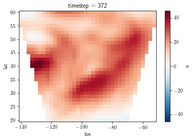
As for pandas, xarray comes with plotting functions. The plot depends on the dimension of the fields:

• 1D: curve

• 2D: pcolormesh

• 3D, 4D, … : histogram

data = xr.open_dataset('data/UV500storm.nc')
data

<xarray.Dataset>
Dimensions:   (lat: 33, lon: 36, timestep: 1)
Coordinates:
  * lat       (lat) float32 20.0 21.25 22.5 23.75 25.0 ... 56.25 57.5 58.75 60.0
  * lon       (lon) float32 -140.0 -137.5 -135.0 -132.5 ... -57.5 -55.0 -52.5
  * timestep  (timestep) int32 372
Data variables:
    reftime   |S20 b'1996 01 05 00:00'
    v         (timestep, lat, lon) float32 nan nan nan nan ... 54.32 49.82 44.32
    u         (timestep, lat, lon) float32 nan nan nan nan ... 7.713 8.213 9.713
Attributes:
    history:  Thu Jul 21 16:12:12 2016: ncks -A U500storm.nc V500storm.nc\nTh...
    NCO:      4.4.2

l = data['u'].isel(timestep=0).plot()

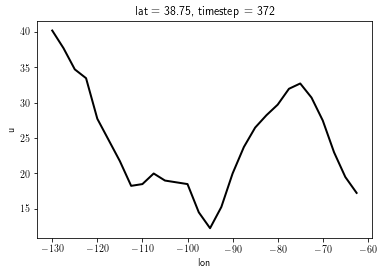
l = data['u'].isel(timestep=0, lat=15).plot()

Mathematical operations

As for pandas, xarray comes with mathematical operations.

data = xr.open_mfdataset('data/*ISAS*', combine='by_coords')

To compute the mean over the entire dataset:

data.mean()

<xarray.Dataset>
Dimensions:  ()
Data variables:
    TEMP     float32 dask.array<chunksize=(), meta=np.ndarray>

To compute the mean along time dimension:

data.mean(dim='time')

<xarray.Dataset>
Dimensions:  (depth: 152)
Coordinates:
  * depth    (depth) float32 0.0 3.0 5.0 10.0 ... 1.96e+03 1.98e+03 2e+03
Data variables:
    TEMP     (depth) float32 dask.array<chunksize=(152,), meta=np.ndarray>

Mean over the depth dimension:

data.mean(dim='depth')

<xarray.Dataset>
Dimensions:  (time: 4)
Coordinates:
  * time     (time) datetime64[ns] 2012-01-15 2012-02-15 2012-03-15 2012-04-15
Data variables:
    TEMP     (time) float32 dask.array<chunksize=(1,), meta=np.ndarray>

Contrary to numpy eager evaluations, xarray performs lazy operations. As indicated on the xarray website:

Operations queue up a series of tasks mapped over blocks, and no computation is performed until you actually ask values to be computed (e.g., to print results to your screen or write to disk)

To force the computation, the compute and/or load methods must be used. Let’s compare the outputs below:

data['TEMP'].mean(dim='time')

<xarray.DataArray 'TEMP' (depth: 152)>
dask.array<mean_agg-aggregate, shape=(152,), dtype=float32, chunksize=(152,), chunktype=numpy.ndarray>
Coordinates:
  * depth    (depth) float32 0.0 3.0 5.0 10.0 ... 1.96e+03 1.98e+03 2e+03

data['TEMP'].mean(dim='time').compute()

<xarray.DataArray 'TEMP' (depth: 152)>
array([28.292002 , 28.27325  , 28.25     , 28.232248 , 28.216    ,
       28.1895   , 28.14475  , 28.1115   , 28.089    , 28.061497 ,
       27.9785   , 27.86825  , 27.706749 , 27.5455   , 27.37575  ,
       27.187498 , 27.0145   , 26.845251 , 26.65725  , 26.47975  ,
       26.300251 , 26.0765   , 25.755249 , 25.4485   , 25.126    ,
       24.78375  , 24.461    , 24.11975  , 23.7695   , 23.343248 ,
       22.948502 , 22.54125  , 22.131    , 21.701248 , 21.247501 ,
       20.817501 , 20.380499 , 19.909    , 19.467499 , 19.02     ,
       18.53825  , 18.0675   , 17.5955   , 17.04475  , 16.568    ,
       16.05925  , 15.553499 , 15.09725  , 14.63025  , 14.14725  ,
       13.635249 , 13.13725  , 12.675499 , 12.21725  , 11.77075  ,
       11.3205   , 10.8885   , 10.518499 , 10.15325  ,  9.795    ,
        9.4395   ,  9.1145   ,  8.85225  ,  8.580999 ,  8.3245   ,
        8.07675  ,  7.8415   ,  7.63525  ,  7.43375  ,  7.23325  ,
        7.0390005,  6.8665   ,  6.71575  ,  6.5675   ,  6.43225  ,
        6.2975   ,  6.17     ,  6.0575   ,  5.9509997,  5.8425   ,
        5.7382503,  5.6480002,  5.5719995,  5.4975   ,  5.42175  ,
        5.34825  ,  5.27975  ,  5.21525  ,  5.1465   ,  5.07925  ,
        5.01725  ,  4.94625  ,  4.8315   ,  4.7165   ,  4.6045   ,
        4.4805   ,  4.36025  ,  4.2535   ,  4.1505   ,  4.0602503,
        3.9720001,  3.8920002,  3.81175  ,  3.738    ,  3.6685   ,
        3.59775  ,  3.53025  ,  3.4675   ,  3.409    ,  3.3554997,
        3.3115   ,  3.2615001,  3.2140002,  3.1664999,  3.12425  ,
        3.0805001,  3.038    ,  2.99825  ,  2.9597497,  2.92275  ,
        2.88575  ,  2.8477502,  2.81425  ,  2.7842498,  2.7525   ,
        2.72125  ,  2.69175  ,  2.66325  ,  2.63925  ,  2.61625  ,
        2.5945   ,  2.5705   ,  2.549    ,  2.527    ,  2.50675  ,
        2.4875   ,  2.46925  ,  2.4507499,  2.43275  ,  2.4145   ,
        2.39675  ,  2.3785   ,  2.3617501,  2.3445   ,  2.32725  ,
        2.3095002,  2.2925   ,  2.27625  ,  2.25875  ,  2.2437499,
        2.2265   ,  2.22025  ], dtype=float32)
Coordinates:
  * depth    (depth) float32 0.0 3.0 5.0 10.0 ... 1.96e+03 1.98e+03 2e+03

In the first output, no values are displayed. The mean has not been computed yet. In the second output, the effective mean values are shown because computation has been forced using compute.

Group-by operations

The groupby methods allows to easily perform operations on indepedent groups. For instance, to compute temporal (yearly, monthly, seasonal) means:

data.groupby('time.month').mean(dim='time')

<xarray.Dataset>
Dimensions:  (month: 4, depth: 152)
Coordinates:
  * depth    (depth) float32 0.0 3.0 5.0 10.0 ... 1.96e+03 1.98e+03 2e+03
  * month    (month) int64 1 2 3 4
Data variables:
    TEMP     (month, depth) float32 dask.array<chunksize=(1, 152), meta=np.ndarray>

data.groupby('time.year').mean(dim='time')

<xarray.Dataset>
Dimensions:  (year: 1, depth: 152)
Coordinates:
  * depth    (depth) float32 0.0 3.0 5.0 10.0 ... 1.96e+03 1.98e+03 2e+03
  * year     (year) int64 2012
Data variables:
    TEMP     (year, depth) float32 dask.array<chunksize=(1, 152), meta=np.ndarray>

data.groupby('time.season').mean(dim='time')

<xarray.Dataset>
Dimensions:  (season: 2, depth: 152)
Coordinates:
  * depth    (depth) float32 0.0 3.0 5.0 10.0 ... 1.96e+03 1.98e+03 2e+03
  * season   (season) object 'DJF' 'MAM'
Data variables:
    TEMP     (season, depth) float32 dask.array<chunksize=(1, 152), meta=np.ndarray>

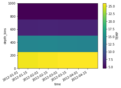
Defining discrete binning (for depth intervals for instance) is done by using the groupby_bins method.

depth_bins = np.arange(0, 1000 + 250, 250)
depth_bins

array([   0,  250,  500,  750, 1000])

zmean = data.groupby_bins('depth', depth_bins).mean(dim='depth')
zmean

<xarray.Dataset>
Dimensions:     (depth_bins: 4, time: 4)
Coordinates:
  * depth_bins  (depth_bins) object (0, 250] (250, 500] (500, 750] (750, 1000]
  * time        (time) datetime64[ns] 2012-01-15 2012-02-15 ... 2012-04-15
Data variables:
    TEMP        (depth_bins, time) float32 dask.array<chunksize=(1, 1), meta=np.ndarray>

import matplotlib.pyplot as plt
plt.rcParams['text.usetex'] = False
cs = zmean['TEMP'].plot()

Let’s reload the ISAS dataset

data = xr.open_mfdataset('data/*ISAS*', combine='by_coords').isel(time=0)
data

<xarray.Dataset>
Dimensions:  (depth: 152)
Coordinates:
  * depth    (depth) float32 0.0 3.0 5.0 10.0 ... 1.96e+03 1.98e+03 2e+03
    time     datetime64[ns] 2012-01-15
Data variables:
    TEMP     (depth) float32 dask.array<chunksize=(152,), meta=np.ndarray>
Attributes:
    script:   extract_prof.py
    history:  Thu Jul 14 11:32:10 2016: ncks -O -3 ISAS13_20120115_fld_TEMP.n...
    NCO:      "4.5.5"

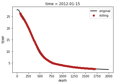
There is the possibility to compute rolling means along the depth dimensions as follows:

datar = data.rolling({'depth': 31}, center=True).mean(dim='depth')
datar

<xarray.Dataset>
Dimensions:  (depth: 152)
Coordinates:
  * depth    (depth) float32 0.0 3.0 5.0 10.0 ... 1.96e+03 1.98e+03 2e+03
    time     datetime64[ns] 2012-01-15
Data variables:
    TEMP     (depth) float64 dask.array<chunksize=(151,), meta=np.ndarray>
Attributes:
    script:   extract_prof.py
    history:  Thu Jul 14 11:32:10 2016: ncks -O -3 ISAS13_20120115_fld_TEMP.n...
    NCO:      "4.5.5"

data['TEMP'].plot(label='original')
datar['TEMP'].plot(label='rolling', marker='o', linestyle='none')
plt.legend()

<matplotlib.legend.Legend at 0x7fd623d7ccd0>

Creating NetCDF

An easy way to write a NetCDF is to create a DataSet object. First, let’sdefine some dummy variables:

import numpy as np
import cftime

nx = 10
ny = 20
ntime = 5
x = np.arange(nx)
y = np.arange(ny)

data = np.random.rand(ntime, ny, nx) - 0.5
data = np.ma.masked_where(data < 0, data)

# converts time into date
time = np.arange(ntime)
date = cftime.num2date(time, 'days since 1900-01-01 00:00:00')

date

array([cftime.DatetimeGregorian(1900, 1, 1, 0, 0, 0, 0, has_year_zero=False),
       cftime.DatetimeGregorian(1900, 1, 2, 0, 0, 0, 0, has_year_zero=False),
       cftime.DatetimeGregorian(1900, 1, 3, 0, 0, 0, 0, has_year_zero=False),
       cftime.DatetimeGregorian(1900, 1, 4, 0, 0, 0, 0, has_year_zero=False),
       cftime.DatetimeGregorian(1900, 1, 5, 0, 0, 0, 0, has_year_zero=False)],
      dtype=object)

data.shape

(5, 20, 10)

First, init an empty Dataset object by calling the xarray.Dataset method.

ds = xr.Dataset()

Then, add to the dataset the variables and coordinates. Note that they should be provided as a tuple that contains two elements:

• A list of dimension names

• The numpy array

ds['data'] = (['time', 'y', 'x'], data)
ds['x'] = (['x'], x)
ds['y'] = (['y'], y)
ds['time'] = (['time'], date)
ds

<xarray.Dataset>
Dimensions:  (time: 5, y: 20, x: 10)
Coordinates:
  * x        (x) int64 0 1 2 3 4 5 6 7 8 9
  * y        (y) int64 0 1 2 3 4 5 6 7 8 9 10 11 12 13 14 15 16 17 18 19
  * time     (time) object 1900-01-01 00:00:00 ... 1900-01-05 00:00:00
Data variables:
    data     (time, y, x) float64 nan nan nan 0.1934 ... 0.07791 0.2112 nan nan

Then, add global and variable attributes to the dataset as follows:

import os
from datetime import datetime

# Set file global attributes (file directory name + date)
ds.attrs['script'] = os.getcwd()
ds.attrs['date'] = str(datetime.today())

ds['data'].attrs['description'] = 'Random draft'
ds

<xarray.Dataset>
Dimensions:  (time: 5, y: 20, x: 10)
Coordinates:
  * x        (x) int64 0 1 2 3 4 5 6 7 8 9
  * y        (y) int64 0 1 2 3 4 5 6 7 8 9 10 11 12 13 14 15 16 17 18 19
  * time     (time) object 1900-01-01 00:00:00 ... 1900-01-05 00:00:00
Data variables:
    data     (time, y, x) float64 nan nan nan 0.1934 ... 0.07791 0.2112 nan nan
Attributes:
    script:   /home/barrier/Work/scientific_communication/seminaires_pomm/pyt...
    date:     2021-10-21 16:12:37.555231

Finally, create the NetCDF file by using the to_netcdf method.

ds.to_netcdf('data/example.nc', unlimited_dims='time', format='NETCDF4')

Note that xarray automatically writes the _FillValue attribute and the time:units attributes.

previous

CSV

next

Cartography