CSV
Reading, writting and analysing CSV files is achived by using the pandas library.
Opening a CSV
The reading of CSV files is done by using the read_csv method.
import pandas as pd

data = pd.read_csv('./data/nina34.csv',
                   delim_whitespace=True,  # use spaces as delimiter
                   skipfooter=3,   # skips the last 2 lines
                   na_values=-99.99,  # sets missing values
                   engine='python'  # sets engine to Python (default C does not support skip footer)
                   )
data
| JAN | FEB | MAR | APR | MAY | JUN | JUL | AUG | SEP | OCT | NOV | DEC | |
|---|---|---|---|---|---|---|---|---|---|---|---|---|
| 1948 | NaN | NaN | NaN | NaN | NaN | NaN | NaN | NaN | NaN | NaN | NaN | NaN |
| 1949 | NaN | NaN | NaN | NaN | NaN | NaN | NaN | NaN | NaN | NaN | NaN | NaN |
| 1950 | 24.55 | 25.06 | 25.87 | 26.28 | 26.18 | 26.46 | 26.29 | 25.88 | 25.74 | 25.69 | 25.47 | 25.29 |
| 1951 | 25.24 | 25.71 | 26.90 | 27.58 | 27.92 | 27.73 | 27.60 | 27.02 | 27.23 | 27.20 | 27.25 | 26.91 |
| 1952 | 26.67 | 26.74 | 27.17 | 27.80 | 27.79 | 27.18 | 26.53 | 26.30 | 26.36 | 26.26 | 25.92 | 26.21 |
| ... | ... | ... | ... | ... | ... | ... | ... | ... | ... | ... | ... | ... |
| 2016 | 29.11 | 29.01 | 28.90 | 28.72 | 28.23 | 27.69 | 26.82 | 26.28 | 26.14 | 25.98 | 25.94 | 26.10 |
| 2017 | 26.12 | 26.67 | 27.32 | 28.03 | 28.30 | 28.06 | 27.54 | 26.70 | 26.29 | 26.15 | 25.74 | 25.62 |
| 2018 | 25.57 | 25.97 | 26.48 | 27.31 | 27.73 | 27.77 | 27.42 | 26.94 | 27.19 | 27.62 | 27.61 | 27.49 |
| 2019 | 27.19 | 27.46 | 28.09 | 28.44 | 28.48 | 28.18 | 27.64 | 26.90 | 26.75 | 27.20 | 27.22 | 27.12 |
| 2020 | 27.18 | NaN | NaN | NaN | NaN | NaN | NaN | NaN | NaN | NaN | NaN | NaN |
73 rows × 12 columns
It returns a pandas.DataFrame object.
To get the names of the line and columns:
data.index
Int64Index([1948, 1949, 1950, 1951, 1952, 1953, 1954, 1955, 1956, 1957, 1958,
            1959, 1960, 1961, 1962, 1963, 1964, 1965, 1966, 1967, 1968, 1969,
            1970, 1971, 1972, 1973, 1974, 1975, 1976, 1977, 1978, 1979, 1980,
            1981, 1982, 1983, 1984, 1985, 1986, 1987, 1988, 1989, 1990, 1991,
            1992, 1993, 1994, 1995, 1996, 1997, 1998, 1999, 2000, 2001, 2002,
            2003, 2004, 2005, 2006, 2007, 2008, 2009, 2010, 2011, 2012, 2013,
            2014, 2015, 2016, 2017, 2018, 2019, 2020],
           dtype='int64')
data.columns
Index(['JAN', 'FEB', 'MAR', 'APR', 'MAY', 'JUN', 'JUL', 'AUG', 'SEP', 'OCT',
       'NOV', 'DEC'],
      dtype='object')
To display some lines at the beginning or at the end:
data.head(3)
| JAN | FEB | MAR | APR | MAY | JUN | JUL | AUG | SEP | OCT | NOV | DEC | |
|---|---|---|---|---|---|---|---|---|---|---|---|---|
| 1948 | NaN | NaN | NaN | NaN | NaN | NaN | NaN | NaN | NaN | NaN | NaN | NaN |
| 1949 | NaN | NaN | NaN | NaN | NaN | NaN | NaN | NaN | NaN | NaN | NaN | NaN |
| 1950 | 24.55 | 25.06 | 25.87 | 26.28 | 26.18 | 26.46 | 26.29 | 25.88 | 25.74 | 25.69 | 25.47 | 25.29 |
data.tail(3)
| JAN | FEB | MAR | APR | MAY | JUN | JUL | AUG | SEP | OCT | NOV | DEC | |
|---|---|---|---|---|---|---|---|---|---|---|---|---|
| 2018 | 25.57 | 25.97 | 26.48 | 27.31 | 27.73 | 27.77 | 27.42 | 26.94 | 27.19 | 27.62 | 27.61 | 27.49 |
| 2019 | 27.19 | 27.46 | 28.09 | 28.44 | 28.48 | 28.18 | 27.64 | 26.90 | 26.75 | 27.20 | 27.22 | 27.12 |
| 2020 | 27.18 | NaN | NaN | NaN | NaN | NaN | NaN | NaN | NaN | NaN | NaN | NaN |
Data extraction
To extract data from the DataFrame, you can either
extract one column
use column/row names
use column/row indexes
Extracting one column
To extract a whole column, we can provide a list of column names as follows:
col = data[['JAN', 'FEB']]
col
| JAN | FEB | |
|---|---|---|
| 1948 | NaN | NaN |
| 1949 | NaN | NaN |
| 1950 | 24.55 | 25.06 |
| 1951 | 25.24 | 25.71 |
| 1952 | 26.67 | 26.74 |
| ... | ... | ... |
| 2016 | 29.11 | 29.01 |
| 2017 | 26.12 | 26.67 |
| 2018 | 25.57 | 25.97 |
| 2019 | 27.19 | 27.46 |
| 2020 | 27.18 | NaN |
73 rows × 2 columns
Using names
Extracting data using column and row names is done by using the loc method.
dataex = data.loc[:, ['JAN', 'FEB']]
dataex
| JAN | FEB | |
|---|---|---|
| 1948 | NaN | NaN |
| 1949 | NaN | NaN |
| 1950 | 24.55 | 25.06 |
| 1951 | 25.24 | 25.71 |
| 1952 | 26.67 | 26.74 |
| ... | ... | ... |
| 2016 | 29.11 | 29.01 |
| 2017 | 26.12 | 26.67 |
| 2018 | 25.57 | 25.97 |
| 2019 | 27.19 | 27.46 |
| 2020 | 27.18 | NaN |
73 rows × 2 columns
dataex = data.loc[[1950, 1960], :]
dataex
| JAN | FEB | MAR | APR | MAY | JUN | JUL | AUG | SEP | OCT | NOV | DEC | |
|---|---|---|---|---|---|---|---|---|---|---|---|---|
| 1950 | 24.55 | 25.06 | 25.87 | 26.28 | 26.18 | 26.46 | 26.29 | 25.88 | 25.74 | 25.69 | 25.47 | 25.29 |
| 1960 | 26.27 | 26.29 | 26.98 | 27.49 | 27.68 | 27.24 | 26.88 | 26.70 | 26.44 | 26.22 | 26.26 | 26.22 |
dataex = data.loc[1950:1953, ['JAN', 'FEB']]
dataex
| JAN | FEB | |
|---|---|---|
| 1950 | 24.55 | 25.06 |
| 1951 | 25.24 | 25.71 |
| 1952 | 26.67 | 26.74 |
| 1953 | 26.74 | 27.00 |
Using indexes
Extracting data using column and row names is done by using the iloc method.
dataex = data.iloc[:5, 0]
dataex
1948      NaN
1949      NaN
1950    24.55
1951    25.24
1952    26.67
Name: JAN, dtype: float64
dataex = data.iloc[2, :]
dataex
JAN    24.55
FEB    25.06
MAR    25.87
APR    26.28
MAY    26.18
JUN    26.46
JUL    26.29
AUG    25.88
SEP    25.74
OCT    25.69
NOV    25.47
DEC    25.29
Name: 1950, dtype: float64
dataex = data.iloc[slice(2, 6), [0, 1]]
dataex
| JAN | FEB | |
|---|---|---|
| 1950 | 24.55 | 25.06 |
| 1951 | 25.24 | 25.71 |
| 1952 | 26.67 | 26.74 |
| 1953 | 26.74 | 27.00 |
dataex = data.iloc[slice(2, 6), :].loc[:, ['OCT', 'NOV']]
dataex
| OCT | NOV | |
|---|---|---|
| 1950 | 25.69 | 25.47 |
| 1951 | 27.20 | 27.25 |
| 1952 | 26.26 | 25.92 |
| 1953 | 26.87 | 26.88 |
Extracting data arrays
To extract the data arrays, use the values attributes.
array = data.values
array.shape
(73, 12)
Plotting
pandas comes with some functions to draw quick plots.
import matplotlib.pyplot as plt
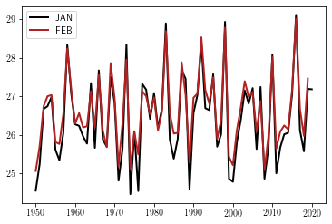
l = data.loc[:, ['JAN', 'FEB']].plot()
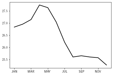
l = data.loc[1970, :].plot()
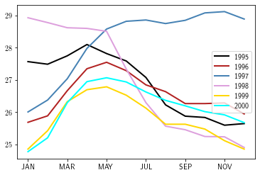
l = data.T.loc[:, 1995:2000].plot()
Creating dataframes
To create a data frame is done by using the pandas.DataFrame method.
import numpy as np

# init a date object: 10 elements with a 1h interval
date = pd.date_range('1/1/2012', periods=10, freq='H')

x = np.arange(10)
y = np.arange(10)*0.5
cat = ['A']*2 + ['C'] + ['A'] + 3*['B'] + ['C'] + ['D'] + ['A']

data = pd.DataFrame({'xvalue': x,
                     'yvalue': y,
                     'cat': cat},
                     index=date)
data
| xvalue | yvalue | cat | |
|---|---|---|---|
| 2012-01-01 00:00:00 | 0 | 0.0 | A |
| 2012-01-01 01:00:00 | 1 | 0.5 | A |
| 2012-01-01 02:00:00 | 2 | 1.0 | C |
| 2012-01-01 03:00:00 | 3 | 1.5 | A |
| 2012-01-01 04:00:00 | 4 | 2.0 | B |
| 2012-01-01 05:00:00 | 5 | 2.5 | B |
| 2012-01-01 06:00:00 | 6 | 3.0 | B |
| 2012-01-01 07:00:00 | 7 | 3.5 | C |
| 2012-01-01 08:00:00 | 8 | 4.0 | D |
| 2012-01-01 09:00:00 | 9 | 4.5 | A |
Mathematical operations
Mathematical operations can be done by using the available pandas methods. Note that it is done only on numerical types. By default, the mean over all the rows is performed:
datam = data.loc[:, ['xvalue', 'yvalue']].mean()
datam
xvalue    4.50
yvalue    2.25
dtype: float64
But you can also compute means over columns:
# mean over the second dimension (columns)
datam = data.loc[:, ['xvalue', 'yvalue']].mean(axis=1)
datam
2012-01-01 00:00:00    0.00
2012-01-01 01:00:00    0.75
2012-01-01 02:00:00    1.50
2012-01-01 03:00:00    2.25
2012-01-01 04:00:00    3.00
2012-01-01 05:00:00    3.75
2012-01-01 06:00:00    4.50
2012-01-01 07:00:00    5.25
2012-01-01 08:00:00    6.00
2012-01-01 09:00:00    6.75
Freq: H, dtype: float64
There is also the possibility to do some treatments depending on the value of a caterogical variable (here, the column called cat).
data_sorted = data.sort_values(by="cat")
data_sorted
| xvalue | yvalue | cat | |
|---|---|---|---|
| 2012-01-01 00:00:00 | 0 | 0.0 | A |
| 2012-01-01 01:00:00 | 1 | 0.5 | A |
| 2012-01-01 03:00:00 | 3 | 1.5 | A |
| 2012-01-01 09:00:00 | 9 | 4.5 | A |
| 2012-01-01 04:00:00 | 4 | 2.0 | B |
| 2012-01-01 05:00:00 | 5 | 2.5 | B |
| 2012-01-01 06:00:00 | 6 | 3.0 | B |
| 2012-01-01 02:00:00 | 2 | 1.0 | C |
| 2012-01-01 07:00:00 | 7 | 3.5 | C |
| 2012-01-01 08:00:00 | 8 | 4.0 | D |
You can count the occurrences:
data.groupby("cat").size()
cat
A    4
B    3
C    2
D    1
dtype: int64
data.groupby("cat").mean()
| xvalue | yvalue | |
|---|---|---|
| cat | ||
| A | 3.25 | 1.625 |
| B | 5.00 | 2.500 |
| C | 4.50 | 2.250 |
| D | 8.00 | 4.000 |
data.groupby("cat").std()
| xvalue | yvalue | |
|---|---|---|
| cat | ||
| A | 4.031129 | 2.015564 |
| B | 1.000000 | 0.500000 |
| C | 3.535534 | 1.767767 |
| D | NaN | NaN |
Writting a CSV
Writting a CSV file is done by calling the DataFrame.to_csv method.
data.to_csv('data/example.csv', sep=';')