Data interpolation
Data interpolation is achieved by using the xesmf library.
It works easily with xarray and dask and therefore can manage parallel computation. As a start, let’s try to interpolate our global SST temperature from the ORCA grid to a regular one.
Reading of the SST
import xarray as xr
import numpy as np
import xesmf as xe

data = xr.open_dataset("data/surface_thetao.nc")
data = data['thetao']
data
<xarray.DataArray 'thetao' (time_counter: 732, olevel: 1, y: 332, x: 362)>
[87974688 values with dtype=float32]
Coordinates:
    nav_lat        (y, x) float32 ...
    nav_lon        (y, x) float32 ...
  * olevel         (olevel) float32 0.5058
    time_centered  (time_counter) object 1958-01-16 12:00:00 ... 2018-12-16 1...
  * time_counter   (time_counter) object 1958-01-16 12:00:00 ... 2018-12-16 1...
Dimensions without coordinates: y, x
Attributes:
    standard_name:       sea_water_conservative_temperature
    long_name:           sea_water_potential_temperature
    units:               degree_C
    online_operation:    average
    interval_operation:  1 month
    interval_write:      1 month
    cell_methods:        time: mean
    cell_measures:       area: area
xarray.DataArray
'thetao'
- time_counter: 732
- olevel: 1
- y: 332
- x: 362
- ...
[87974688 values with dtype=float32]
- nav_lat(y, x)float32...
- standard_name :
- latitude
- long_name :
- Latitude
- units :
- degrees_north
- bounds :
- bounds_nav_lat
[120184 values with dtype=float32]
- nav_lon(y, x)float32...
- standard_name :
- longitude
- long_name :
- Longitude
- units :
- degrees_east
- bounds :
- bounds_nav_lon
[120184 values with dtype=float32]
- olevel(olevel)float320.5058
- name :
- olevel
- long_name :
- Vertical T levels
- units :
- m
- positive :
- down
- bounds :
- olevel_bounds
array([0.50576], dtype=float32)
- time_centered(time_counter)object...
- standard_name :
- time
- long_name :
- Time axis
- time_origin :
- 1958-01-01 00:00:00
- bounds :
- time_centered_bounds
array([cftime.DatetimeNoLeap(1958, 1, 16, 12, 0, 0, 0, has_year_zero=True), cftime.DatetimeNoLeap(1958, 2, 15, 0, 0, 0, 0, has_year_zero=True), cftime.DatetimeNoLeap(1958, 3, 16, 12, 0, 0, 0, has_year_zero=True), ..., cftime.DatetimeNoLeap(2018, 10, 16, 12, 0, 0, 0, has_year_zero=True), cftime.DatetimeNoLeap(2018, 11, 16, 0, 0, 0, 0, has_year_zero=True), cftime.DatetimeNoLeap(2018, 12, 16, 12, 0, 0, 0, has_year_zero=True)], dtype=object) - time_counter(time_counter)object1958-01-16 12:00:00 ... 2018-12-...
- axis :
- T
- standard_name :
- time
- long_name :
- Time axis
- time_origin :
- 1958-01-01 00:00:00
- bounds :
- time_counter_bounds
array([cftime.DatetimeNoLeap(1958, 1, 16, 12, 0, 0, 0, has_year_zero=True),
       cftime.DatetimeNoLeap(1958, 2, 15, 0, 0, 0, 0, has_year_zero=True),
       cftime.DatetimeNoLeap(1958, 3, 16, 12, 0, 0, 0, has_year_zero=True),
       ...,
       cftime.DatetimeNoLeap(2018, 10, 16, 12, 0, 0, 0, has_year_zero=True),
       cftime.DatetimeNoLeap(2018, 11, 16, 0, 0, 0, 0, has_year_zero=True),
       cftime.DatetimeNoLeap(2018, 12, 16, 12, 0, 0, 0, has_year_zero=True)],
      dtype=object)
- standard_name :
- sea_water_conservative_temperature
- long_name :
- sea_water_potential_temperature
- units :
- degree_C
- online_operation :
- average
- interval_operation :
- 1 month
- interval_write :
- 1 month
- cell_methods :
- time: mean
- cell_measures :
- area: area
Initialisation of the output grid
Then, a Dataset object that contains the output grid must be created
dsout = xr.Dataset()
dsout['lon'] = (['lon'], np.arange(-179, 179 + 1))
dsout['lat'] = (['lat'], np.arange(-89, 89 + 1))
dsout
<xarray.Dataset>
Dimensions:  (lon: 359, lat: 179)
Coordinates:
  * lon      (lon) int64 -179 -178 -177 -176 -175 -174 ... 175 176 177 178 179
  * lat      (lat) int64 -89 -88 -87 -86 -85 -84 -83 ... 83 84 85 86 87 88 89
Data variables:
    *empty*
xarray.Dataset
- lon: 359
- lat: 179
- lon(lon)int64-179 -178 -177 -176 ... 177 178 179
array([-179, -178, -177, ..., 177, 178, 179])
- lat(lat)int64-89 -88 -87 -86 -85 ... 86 87 88 89
array([-89, -88, -87, -86, -85, -84, -83, -82, -81, -80, -79, -78, -77, -76,
       -75, -74, -73, -72, -71, -70, -69, -68, -67, -66, -65, -64, -63, -62,
       -61, -60, -59, -58, -57, -56, -55, -54, -53, -52, -51, -50, -49, -48,
       -47, -46, -45, -44, -43, -42, -41, -40, -39, -38, -37, -36, -35, -34,
       -33, -32, -31, -30, -29, -28, -27, -26, -25, -24, -23, -22, -21, -20,
       -19, -18, -17, -16, -15, -14, -13, -12, -11, -10,  -9,  -8,  -7,  -6,
        -5,  -4,  -3,  -2,  -1,   0,   1,   2,   3,   4,   5,   6,   7,   8,
         9,  10,  11,  12,  13,  14,  15,  16,  17,  18,  19,  20,  21,  22,
        23,  24,  25,  26,  27,  28,  29,  30,  31,  32,  33,  34,  35,  36,
        37,  38,  39,  40,  41,  42,  43,  44,  45,  46,  47,  48,  49,  50,
        51,  52,  53,  54,  55,  56,  57,  58,  59,  60,  61,  62,  63,  64,
        65,  66,  67,  68,  69,  70,  71,  72,  73,  74,  75,  76,  77,  78,
        79,  80,  81,  82,  83,  84,  85,  86,  87,  88,  89])
Renaming the input coordinates
We also need to insure that the coordinates variables have the same names.
data = data.rename({'nav_lon' : 'lon', 'nav_lat' : 'lat'})
data
<xarray.DataArray 'thetao' (time_counter: 732, olevel: 1, y: 332, x: 362)>
[87974688 values with dtype=float32]
Coordinates:
    lat            (y, x) float32 ...
    lon            (y, x) float32 ...
  * olevel         (olevel) float32 0.5058
    time_centered  (time_counter) object 1958-01-16 12:00:00 ... 2018-12-16 1...
  * time_counter   (time_counter) object 1958-01-16 12:00:00 ... 2018-12-16 1...
Dimensions without coordinates: y, x
Attributes:
    standard_name:       sea_water_conservative_temperature
    long_name:           sea_water_potential_temperature
    units:               degree_C
    online_operation:    average
    interval_operation:  1 month
    interval_write:      1 month
    cell_methods:        time: mean
    cell_measures:       area: area
xarray.DataArray
'thetao'
- time_counter: 732
- olevel: 1
- y: 332
- x: 362
- ...
[87974688 values with dtype=float32]
- lat(y, x)float32...
- standard_name :
- latitude
- long_name :
- Latitude
- units :
- degrees_north
- bounds :
- bounds_nav_lat
[120184 values with dtype=float32]
- lon(y, x)float32...
- standard_name :
- longitude
- long_name :
- Longitude
- units :
- degrees_east
- bounds :
- bounds_nav_lon
[120184 values with dtype=float32]
- olevel(olevel)float320.5058
- name :
- olevel
- long_name :
- Vertical T levels
- units :
- m
- positive :
- down
- bounds :
- olevel_bounds
array([0.50576], dtype=float32)
- time_centered(time_counter)object1958-01-16 12:00:00 ... 2018-12-...
- standard_name :
- time
- long_name :
- Time axis
- time_origin :
- 1958-01-01 00:00:00
- bounds :
- time_centered_bounds
array([cftime.DatetimeNoLeap(1958, 1, 16, 12, 0, 0, 0, has_year_zero=True), cftime.DatetimeNoLeap(1958, 2, 15, 0, 0, 0, 0, has_year_zero=True), cftime.DatetimeNoLeap(1958, 3, 16, 12, 0, 0, 0, has_year_zero=True), ..., cftime.DatetimeNoLeap(2018, 10, 16, 12, 0, 0, 0, has_year_zero=True), cftime.DatetimeNoLeap(2018, 11, 16, 0, 0, 0, 0, has_year_zero=True), cftime.DatetimeNoLeap(2018, 12, 16, 12, 0, 0, 0, has_year_zero=True)], dtype=object) - time_counter(time_counter)object1958-01-16 12:00:00 ... 2018-12-...
- axis :
- T
- standard_name :
- time
- long_name :
- Time axis
- time_origin :
- 1958-01-01 00:00:00
- bounds :
- time_counter_bounds
array([cftime.DatetimeNoLeap(1958, 1, 16, 12, 0, 0, 0, has_year_zero=True),
       cftime.DatetimeNoLeap(1958, 2, 15, 0, 0, 0, 0, has_year_zero=True),
       cftime.DatetimeNoLeap(1958, 3, 16, 12, 0, 0, 0, has_year_zero=True),
       ...,
       cftime.DatetimeNoLeap(2018, 10, 16, 12, 0, 0, 0, has_year_zero=True),
       cftime.DatetimeNoLeap(2018, 11, 16, 0, 0, 0, 0, has_year_zero=True),
       cftime.DatetimeNoLeap(2018, 12, 16, 12, 0, 0, 0, has_year_zero=True)],
      dtype=object)
- standard_name :
- sea_water_conservative_temperature
- long_name :
- sea_water_potential_temperature
- units :
- degree_C
- online_operation :
- average
- interval_operation :
- 1 month
- interval_write :
- 1 month
- cell_methods :
- time: mean
- cell_measures :
- area: area
Creating the interpolator
When this is done, the interpolator object can be created as follows:
regridder = xe.Regridder(data, dsout, 'bilinear', ignore_degenerate=True, reuse_weights=False, periodic=True, filename='weights.nc')
regridder
/home/barrier/Softwares/anaconda3/lib/python3.7/site-packages/xarray/core/dataarray.py:789: FutureWarning: elementwise comparison failed; returning scalar instead, but in the future will perform elementwise comparison
  return key in self.data
xESMF Regridder
Regridding algorithm:       bilinear
Weight filename:            weights.nc
Reuse pre-computed weights? False
Input grid shape:           (332, 362)
Output grid shape:          (179, 359)
Periodic in longitude?      True
Note that the ignore_degenerate argument is necessary for handling the ORCA grid.
Interpolating the data set
dataout = regridder(data)
/home/barrier/Softwares/anaconda3/lib/python3.7/site-packages/xesmf/frontend.py:534: FutureWarning: ``output_sizes`` should be given in the ``dask_gufunc_kwargs`` parameter. It will be removed as direct parameter in a future version.
  keep_attrs=keep_attrs,
Comparing the results
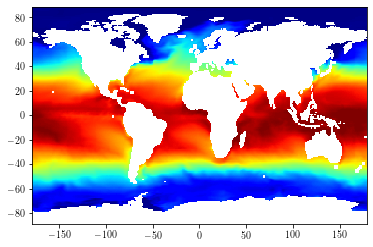
Let’s display the original SST values for the first time-step
import matplotlib.pyplot as plt

mesh = xr.open_dataset("data/mesh_mask_eORCA1_v2.2.nc")
lonf = mesh['glamf'].data[0]
latf = mesh['gphif'].data[0]

toplot = data.isel(time_counter=0, olevel=0).data
cs = plt.pcolormesh(lonf, latf, toplot[1:, 1:], cmap=plt.cm.jet)
cs.set_clim(-2, 30)
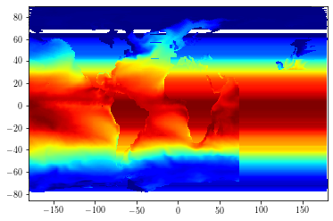
toplot = dataout.isel(time_counter=0, olevel=0).data
cs = plt.pcolormesh(dataout['lon'], dataout['lat'], toplot[1:, 1:], cmap=plt.cm.jet)
cs.set_clim(-2, 30)