Maps
Drawing maps can be achieved by using the cartopy library, which can be used with matplotlib.
Install
Since it is not a standard library, it needs to be installed. It is best to do it using conda, since it needs external C libraries. To install it, type in a terminal:
conda install cartopy
Map initialisation
Maps are initialized by using the pyplot.axes with a projection argument that defines the Coordinate Reference System, i.e. a projection system. The list of available projections can be found here.
import cartopy.crs as ccrs
import matplotlib.pyplot as plt
import numpy as np
plt.rcParams['text.usetex'] = False
fig = plt.figure()
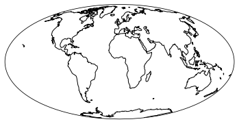
ax = plt.axes(projection=ccrs.Mollweide())
l = ax.coastlines() # add coastlines
import cartopy.crs as ccrs
import matplotlib.pyplot as plt
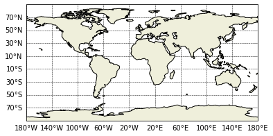
fig = plt.figure()
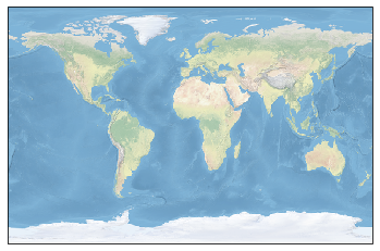
ax = plt.axes(projection=ccrs.PlateCarree())
l = ax.stock_img()
Specifying map limits
Map limits can be specified using the set_extent method. It takes as argument the limits of the maps and eventually a crs object, specifying the coordinate system used to specify the limits.
In most cases, limits are defined in geographical coordinates. Thus the crs argument must be equal to ccrs.PlateCarree()
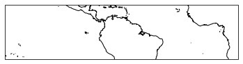
fig = plt.figure()
ax = plt.axes(projection=ccrs.PlateCarree())
ax.set_extent([-150, 20, -20, 20], crs=ccrs.PlateCarree())
l = ax.coastlines()
Adding map features
In order to add features to the map (land color, ocean colors, etc.), use the cartopy.feature interface.
Features should be added to the current axes by using the add_feature method.
Using predefined features
Some features, such as lands ans oceans, coastlines, country borders and lakes are avaiblable. For instance, land mask is accessed as cfeature.LAND.
import cartopy.crs as ccrs
import cartopy.feature as cfeature
import matplotlib.pyplot as plt
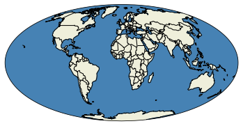
fig = plt.figure()
ax = plt.axes(projection=ccrs.Mollweide())
ax.add_feature(cfeature.LAND, facecolor=cfeature.COLORS['land'])
ax.add_feature(cfeature.COASTLINE, edgecolor='k')
ax.add_feature(cfeature.BORDERS)
ax.add_feature(cfeature.OCEAN, color='SteelBlue')
plt.show()
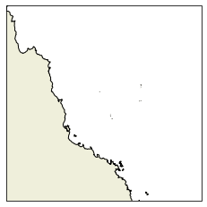
There is the possibility to control the resolution of the default features you by using the with_scale argument.
latc = -18 + 56/60.+ 15/(60 * 60)
lonc = 148 + 5/60 + 45/(60*60)

fig = plt.figure()
ax = plt.axes(projection=ccrs.PlateCarree())
ax.set_extent([lonc - 5, lonc + 5, latc - 5, latc + 5], ccrs.PlateCarree())
ax.add_feature(cfeature.LAND.with_scale('10m'), facecolor=cfeature.COLORS['land'])
ax.add_feature(cfeature.COASTLINE.with_scale('10m'), edgecolor='k')
plt.show()
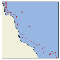
Using Natural Earth Data data
It is also possible to use include other features from naturalearthdata by using the
cartopy.feature.NaturalEarthFeature interface. For instance, one can add coral reefs as follows:
# Create a feature for reefs image
reefs = cfeature.NaturalEarthFeature(
    category='physical',
    name='reefs',
    scale='10m',
    edgecolor='face',
    facecolor='FireBrick'
)

latc = -18 + 56/60.+ 15/(60 * 60)
lonc = 148 + 5/60 + 45/(60*60)

fig = plt.figure()
ax = plt.axes(projection=ccrs.PlateCarree())
ax.set_extent([lonc - 5, lonc + 5, latc - 5, latc + 5], ccrs.PlateCarree())
ax.add_feature(cfeature.LAND)
ax.add_feature(cfeature.OCEAN)
ax.add_feature(reefs)
ax.coastlines(resolution='50m')
plt.show()
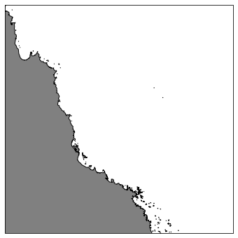
Using GSHSS features
There is also the possibility to use GSHSS features:
fig = plt.figure(figsize=(6, 6))
ax = plt.axes(projection=ccrs.PlateCarree())
ax.set_xlim(lonc - 5, lonc + 5)
ax.set_ylim(latc - 5, latc + 5)
ax.add_feature(cfeature.GSHHSFeature(scale='intermediate', levels=[1], facecolor='gray', edgecolor='k'))
plt.show()
Labeling
Informations about how to add grid labels are provided here: https://scitools.org.uk/cartopy/docs/v0.13/matplotlib/gridliner.html
Here is a small example on how to do it.
First, you need to import some modules and to define a dictionary containing the map parameters:
from cartopy.mpl.gridliner import LONGITUDE_FORMATTER, LATITUDE_FORMATTER
import matplotlib.ticker as mticker

# definition of grid params
gridparams = {'crs': ccrs.PlateCarree(central_longitude=0),
              'draw_labels':True, 'linewidth':0.5,
              'color':'k', 'alpha':1, 'linestyle':'--'}
Then you can use the ax.gridlines method with the **gridparams method to add the grid lines.
fig = plt.figure()
ax = plt.axes(projection=ccrs.PlateCarree())
ax.add_feature(cfeature.LAND, zorder=1)
ax.add_feature(cfeature.COASTLINE, zorder=2)
gl = ax.gridlines(**gridparams, zorder=0)
If you want to control which labels are drawn, and where, you can modify the values of the gl object as follows:
fig = plt.figure()
ax = plt.axes(projection=ccrs.PlateCarree())
ax.add_feature(cfeature.LAND, zorder=1)
ax.add_feature(cfeature.COASTLINE, zorder=2)
gl = ax.gridlines(**gridparams, zorder=0)
gl.xlabels_top = False
gl.ylabels_right = False
gl.xlocator = mticker.FixedLocator(np.arange(-180, 180 + 40, 40))
gl.ylocator = mticker.FixedLocator(np.arange(-90, 90 + 20, 20))
gl.xformatter = LONGITUDE_FORMATTER
gl.yformatter = LATITUDE_FORMATTER
/home/barrier/Softwares/anaconda3/lib/python3.7/site-packages/cartopy/mpl/gridliner.py:451: UserWarning: The .xlabels_top attribute is deprecated. Please use .top_labels to toggle visibility instead.
  warnings.warn('The .xlabels_top attribute is deprecated. Please '
/home/barrier/Softwares/anaconda3/lib/python3.7/site-packages/cartopy/mpl/gridliner.py:487: UserWarning: The .ylabels_right attribute is deprecated. Please use .right_labels to toggle visibility instead.
  warnings.warn('The .ylabels_right attribute is deprecated. Please '
Plotting data
Examples on how to plot data using Cartopy are provided here.
Basically, the same methods as in Matplotlib are used, except that a transform argument must be set equal to the projection used in the input data.
In most cases, the data are provided in geographical coordinates. Therefore, the transform argument must be set to ccrs.PlateCarree().
First, let’s load a dataset:
import xarray as xr
import numpy as np

data = xr.open_dataset('../io/data/UV500storm.nc')
lon = data['lon'].values
lat = data['lat'].values
u = data['u'].values[0]
v = data['v'].values[0]
u = np.ma.masked_where(np.abs(u) > 999, u)
v = np.ma.masked_where(np.abs(v) > 999, v)
vel = np.sqrt(u*u + v*v, where=(np.ma.getmaskarray(u) == False))
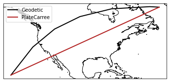
Lines
In order to draw lines that follow geodetic distance, set the transform argument as equal to ccrs.Geodetic().
fig = plt.figure()
ax = plt.axes(projection=ccrs.PlateCarree())
x = [lon.min(), lon.max()]
y = [lat.min(), lat.max()]
ax.plot(x, y, transform=ccrs.Geodetic(), label='Geodetic')
ax.plot(x, y, transform=ccrs.PlateCarree(), label='PlateCarree')
plt.legend()
ax.coastlines()
<cartopy.mpl.feature_artist.FeatureArtist at 0x7fa7deebf790>
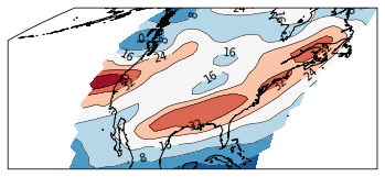
Contours
fig = plt.figure()
ax = plt.axes(projection=ccrs.Mollweide())
cs = plt.contourf(lon, lat, u, transform=ccrs.PlateCarree())
cl = plt.contour(lon, lat, u, transform=ccrs.PlateCarree(), colors='k', linewidths=0.5)
plt.clabel(cl)
ax.coastlines()  # add coastlines
plt.show()
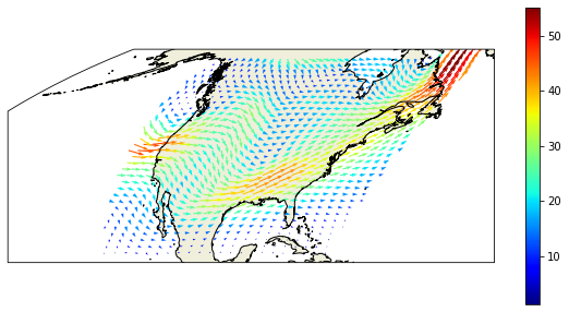
Quivers
import matplotlib

fig = plt.figure(figsize=(10, 10))

ax = plt.axes(projection=ccrs.Mollweide())
cs = plt.quiver(lon, lat, u, v, vel, cmap=plt.cm.jet, transform=ccrs.PlateCarree())
cb = plt.colorbar(cs, shrink=0.5)

ax.coastlines()  # add coastlines
ax.add_feature(cfeature.LAND)
<cartopy.mpl.feature_artist.FeatureArtist at 0x7fa7e55e00d0>
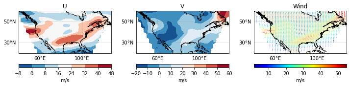
Paneling
Proper paneling can be obtained by using the ImageGrid Matplotlib function in combination with the GeoAxes method (cf. https://scitools.org.uk/cartopy/docs/v0.16/gallery/axes_grid_basic.html)
from mpl_toolkits.axes_grid1 import ImageGrid
from cartopy.mpl.geoaxes import GeoAxes
import cartopy.feature as cfeature

def add_labels(ax, projout):
    gridparams = {'crs': projout,
              'draw_labels':True, 'linewidth':0.5,
              'color':'gray', 'alpha':0.5, 'linestyle':'--'}
    gl = ax.gridlines(**gridparams)
    gl.xlabels_top = False
    gl.ylabels_right = False
    gl.xformatter = LONGITUDE_FORMATTER
    gl.yformatter = LATITUDE_FORMATTER
    gl.xlocator = mticker.FixedLocator(np.arange(-180, 180 + 40, 40))
    gl.ylocator = mticker.FixedLocator(np.arange(-90, 90 + 20, 20))

projout = ccrs.PlateCarree(central_longitude=180)
projin = ccrs.PlateCarree()

fig = plt.figure(figsize=(12, 8))
axes_class = (GeoAxes, dict(map_projection=projout))

axgr = ImageGrid(fig, 111,  axes_class=axes_class, nrows_ncols=(1, 3), axes_pad=(0.7, 0.5), label_mode='',
                cbar_mode='each', cbar_size=0.1, cbar_pad=0.3, cbar_location="bottom", share_all=True)

axcbar = axgr.cbar_axes

for i, ax in enumerate(axgr):
    if i == 0:
        cs = ax.contourf(lon, lat, u, transform=projin)
        ax.set_title('U')
        cb = axcbar[i].colorbar(cs)
    elif i == 1:
        cs = ax.contourf(lon, lat, v, transform=projin)
        cb = axcbar[i].colorbar(cs)
        ax.set_title('V')
    else:
        cs = ax.quiver(lon, lat, u, v, vel, cmap=plt.cm.jet, transform=projin)
        cb = axcbar[i].colorbar(cs)
        ax.set_title('Wind')
    ax.add_feature(cfeature.LAND)  # add coastlines
    ax.add_feature(cfeature.COASTLINE)  # add coastlines
    cb.set_label('m/s')
    add_labels(ax, projout)
/home/barrier/Softwares/anaconda3/lib/python3.7/site-packages/cartopy/mpl/gridliner.py:451: UserWarning: The .xlabels_top attribute is deprecated. Please use .top_labels to toggle visibility instead.
  warnings.warn('The .xlabels_top attribute is deprecated. Please '
/home/barrier/Softwares/anaconda3/lib/python3.7/site-packages/cartopy/mpl/gridliner.py:487: UserWarning: The .ylabels_right attribute is deprecated. Please use .right_labels to toggle visibility instead.
  warnings.warn('The .ylabels_right attribute is deprecated. Please '
Switching from one system to another
The transform_points method can be used to navigate between coordinates systems. It is called as follow:
destCRS.transform_points(sourceCrs, longitudes, latitudes)
For instance, to convert longitudes/latitudes into Mollweide map coordinates:
projin = ccrs.PlateCarree()
projout = ccrs.Mollweide()

N = 10
lone = np.linspace(-180, 180, N)
late = np.full((N), 0)

convert = projout.transform_points(projin, lone, late)
xe = convert[:, 0]
ye = convert[:, 1]
ze = convert[:, 2]
xe,  ye
(array([-18040095.69614736, -14031185.54144795, -10022275.38674853,
         -6013365.23204912,  -2004455.07734971,   2004455.07734971,
          6013365.23204912,  10022275.38674853,  14031185.54144795,
         18040095.69614736]),
 array([0., 0., 0., 0., 0., 0., 0., 0., 0., 0.]))
Note that the transform_vectors can be used to convert vectors from one CRS to another.
Changing map boundary
There is the possibility to change the map bounding box. This is especially usefull if you want to use the Masked Lambert Conformal projection. First, let’s have a look at the LCC projection:
lonw = -80
lone = 40
lats = 10
latn = 75

lon0 = 0.5 * (lone + lonw)
lat0 = 0.5 * (lats + latn)

plt.figure()
proj = ccrs.LambertConformal(central_longitude=lon0)
ax = plt.axes(projection=proj)
ax.set_extent([lonw, lone, lats, latn], ccrs.PlateCarree())
i = ax.coastlines()
ax.add_feature(cfeature.LAND)
<cartopy.mpl.feature_artist.FeatureArtist at 0x7fa7e5405090>
In order to mask it, the boundary polygon needs to be defined in geographical coordinates as a Path object:
import matplotlib.path as mpath
import numpy as np

N = 100
First, we create the array of coordinates for the southern border:
xsouth = np.linspace(lonw, lone, N)
ysouth = np.full((N), lats)
Then, we create the coordinates for the eastern border:
yeast = np.linspace(lats, latn, N)
xeast = np.full((N), lone)
Same thing is repeated for the western and eastern order. Except that the order is reversed.
xnorth = np.linspace(lonw, lone, N)[::-1]
ynorth = np.full((N), latn)

ywest = np.linspace(lats, latn, N)[::-1]
xwest = np.full((N), lonw)
Then, we combine all these coordinates into 1D arrays:
x = np.concatenate([xsouth, xeast, xnorth, xwest])
y = np.concatenate([ysouth, yeast, ynorth, ywest])
We can check that the domain is properly defined:
plt.figure()
proj = ccrs.LambertConformal(central_longitude=lon0)
ax = plt.axes(projection=proj)
ax.set_extent([x.min(), x.max(), y.min(), y.max()], ccrs.PlateCarree())
ax.plot(x, y, transform=ccrs.PlateCarree())
l = ax.coastlines()
l = ax.add_feature(cfeature.LAND)
Now, we convert the x, y arrays into a matplotlib.path.Path object:
path = mpath.Path(np.array([x, y]).T)
Now, the map boundary can be specified using the set_boundary method:
plt.figure()
proj = ccrs.LambertConformal(central_longitude=lon0)
ax = plt.axes(projection=proj)
ax.set_extent([x.min(), x.max(), y.min(), y.max()], ccrs.PlateCarree())
ax.set_boundary(path, transform=ccrs.PlateCarree())
l = ax.coastlines()
l = ax.add_feature(cfeature.LAND)
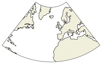
The features must be added after the new boundaries have been set