PyNGL
The PyNGL library is a very powerfull tool for mapping.
Install
To install PyNGL, it is strongly recommended to set-up a virtual environment, as described on the Download section:
conda create --name pyngl
conda activate pyngl
conda install pyngl
conda install pynio
conda install xarray
To use Jupyter Notebook with this environment, type in a terminal:
conda activate pyngl
conda install ipython ipykernel
ipython kernel install --name "pyngl" --user
jupyter notebook &
(source: Medium.com)
General concepts
Workspace
In PyNGL, a figure is called a Workspace. It is opened by using the Ngl.open_wks method.
Draw and Frame
A plot is referred to as a Draw, while a figure page (for instance PDF page) is referred to as a Frame.
Any time a plot is done, a Draw is created on a Frame, then a Frame is added to the Workspace , except if the user decides to keep control on when these actions should be performed (which is highly recommended).
Finally, figures are finalized by calling the Ngl.end method.
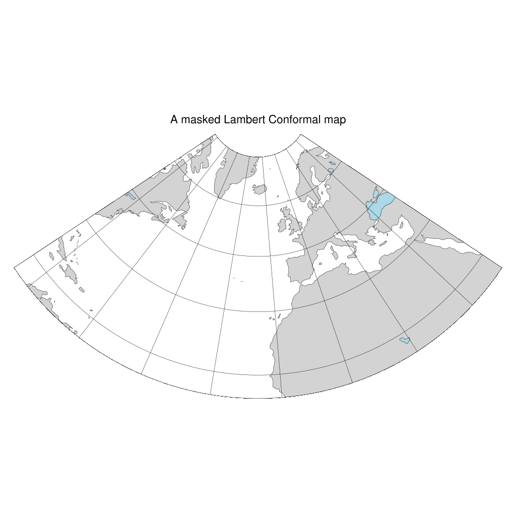
First map
import Ngl
import xarray as xr
import numpy as np

# load the NetCDF file, using the PyNio engine
data = xr.open_dataset('../io/data/UV500storm.nc', engine='pynio')
data = data.isel(timestep=0)

lon = data['lon'].values
lat = data['lat'].values
u = data['u'].to_masked_array()
v = data['v'].to_masked_array()
speed = np.sqrt(u*u+v*v, where=(np.ma.getmaskarray(u) == False))

# open document
wks = Ngl.open_wks("png", "figs/pyngl_examples.png")

# initialisation of the plot resources
res = Ngl.Resources()

# not necessary, just a good habit
res.nglDraw = False  # deactivate drawing
res.nglFrame = False # deactivate page generation

# Set map resources.
res.mpProjection = "LambertConformal" # proj
res.nglMaskLambertConformal = True # masked lamb
res.mpLimitMode = "LatLon"     # limit map via lat/lon
res.mpMinLatF = 10.         # map area
res.mpMaxLatF = 75.         # latitudes
res.mpMinLonF = -80.         # and
res.mpMaxLonF = 40.         # longitudes
res.mpFillOn = True # fill map
res.mpLandFillColor = "LightGray"
res.mpOceanFillColor = -1 # oceans are transparent
res.mpInlandWaterFillColor = "LightBlue" # lakes are light blue
res.tiMainString = "A masked Lambert Conformal map" # plot title
res.tiMainFontHeightF = 0.010  # Font size

# makes the map
m = Ngl.map(wks, res)

# draws the map
Ngl.draw(m)

# add a page to the pdf output
Ngl.frame(wks)

#Ngl.end()
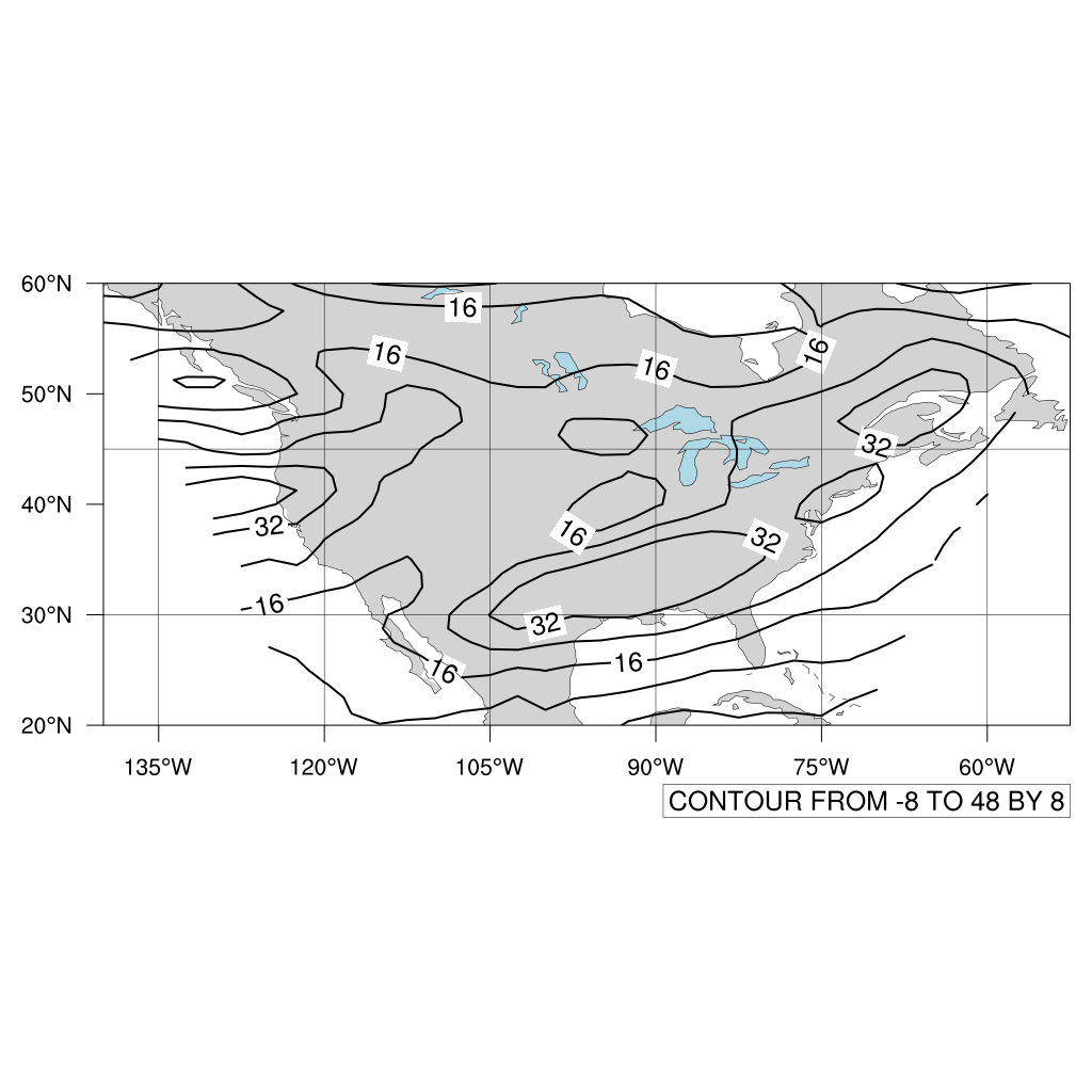
Contour plots
# init the plot resources
res = Ngl.Resources()

# not necessary, just a good habit
res.nglDraw = False
res.nglFrame = False

# Set map resources.
res.mpLimitMode = "LatLon"     # limit map via lat/lon
res.mpMinLatF = lat.min()         # map area
res.mpMaxLatF = lat.max()         # latitudes
res.mpMinLonF = lon.min()         # and
res.mpMaxLonF = lon.max()         # longitudes
res.mpFillOn = True
res.mpLandFillColor = "LightGray"
res.mpOceanFillColor = -1
res.mpInlandWaterFillColor = "LightBlue"

# coordinates for contour plots
res.sfXArray = lon
res.sfYArray = lat

# Set properties for contour lones
res.cnFillOn             = False # no filled contour
res.cnLinesOn            = True # contour lines
res.cnLineLabelsOn       = True # line labels
res.cnLineThicknessF =   4 # contour lines thickness
res.cnLevelSelectionMode = "ExplicitLevels" # plotted levels are set explicitely
res.cnLevels      = np.arange(-8, 48+8, 8) # levels to plot
res.cnInfoLabelOn = True # add the contour info

# draw the contour maps
m = Ngl.contour_map(wks, u, res)

# draws the map
Ngl.draw(m)

# add a page to the pdf output
Ngl.frame(wks)

# ends the plot
# Ngl.end()
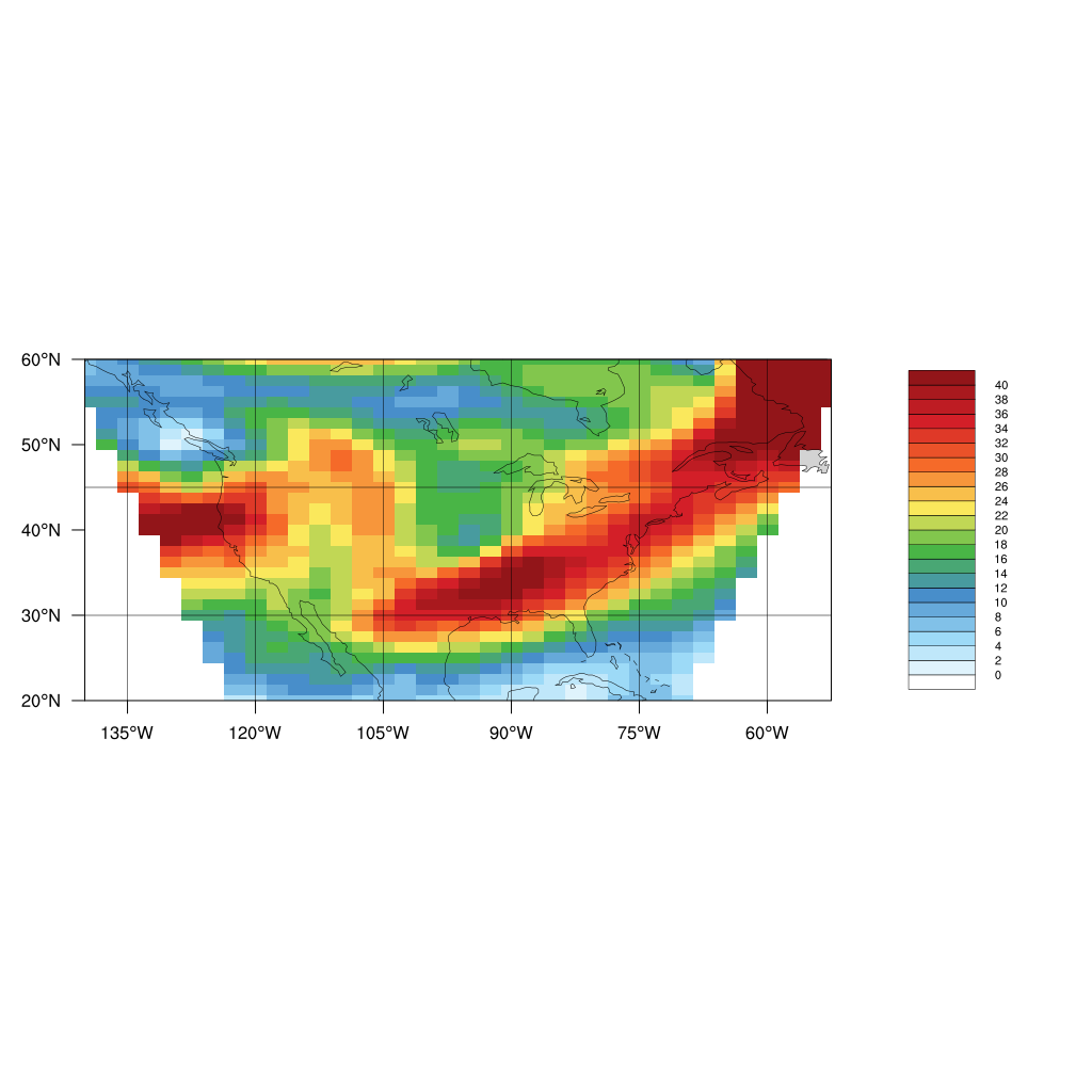
Filled contours
# set the document colormap
resngl = Ngl.Resources()
resngl.wkColorMap = 'WhiteBlueGreenYellowRed'
Ngl.set_values(wks, resngl)

# init the plot resources
res = Ngl.Resources()

# not necessary, just a good habit
res.nglDraw = False
res.nglFrame = False

# Set map resources.
res.mpLimitMode = "LatLon"     # limit map via lat/lon
res.mpMinLatF = lat.min()         # map area
res.mpMaxLatF = lat.max()         # latitudes
res.mpMinLonF = lon.min()         # and
res.mpMaxLonF = lon.max()         # longitudes
res.mpFillOn = True
res.mpLandFillColor = "LightGray"
res.mpOceanFillColor = -1
res.mpInlandWaterFillColor = "LightBlue"

# coordinates for contour plots
res.sfXArray = lon
res.sfYArray = lat

# Set properties for contour lones
res.cnFillOn             = True # no filled contour
res.cnLinesOn            = False # contour lines
res.cnLineLabelsOn = False
res.cnLineThicknessF =   4 # contour lines thickness
res.cnLevelSelectionMode = "ExplicitLevels" # plotted levels are set explicitely
res.cnFillMode = "CellFill"
res.cnLevels      = np.linspace(0, 40, 21) # levels to plot

res.nglSpreadColors = True
res.nglSpreadColorStart = 2
res.nglSpreadColorEnd = 255

# draw the contour maps
m = Ngl.contour_map(wks, speed, res)

# draws the map
Ngl.draw(m)

# add a page to the pdf output
Ngl.frame(wks)

# add the colormap to see the colors
Ngl.draw_colormap(wks)

# Ngl.end()
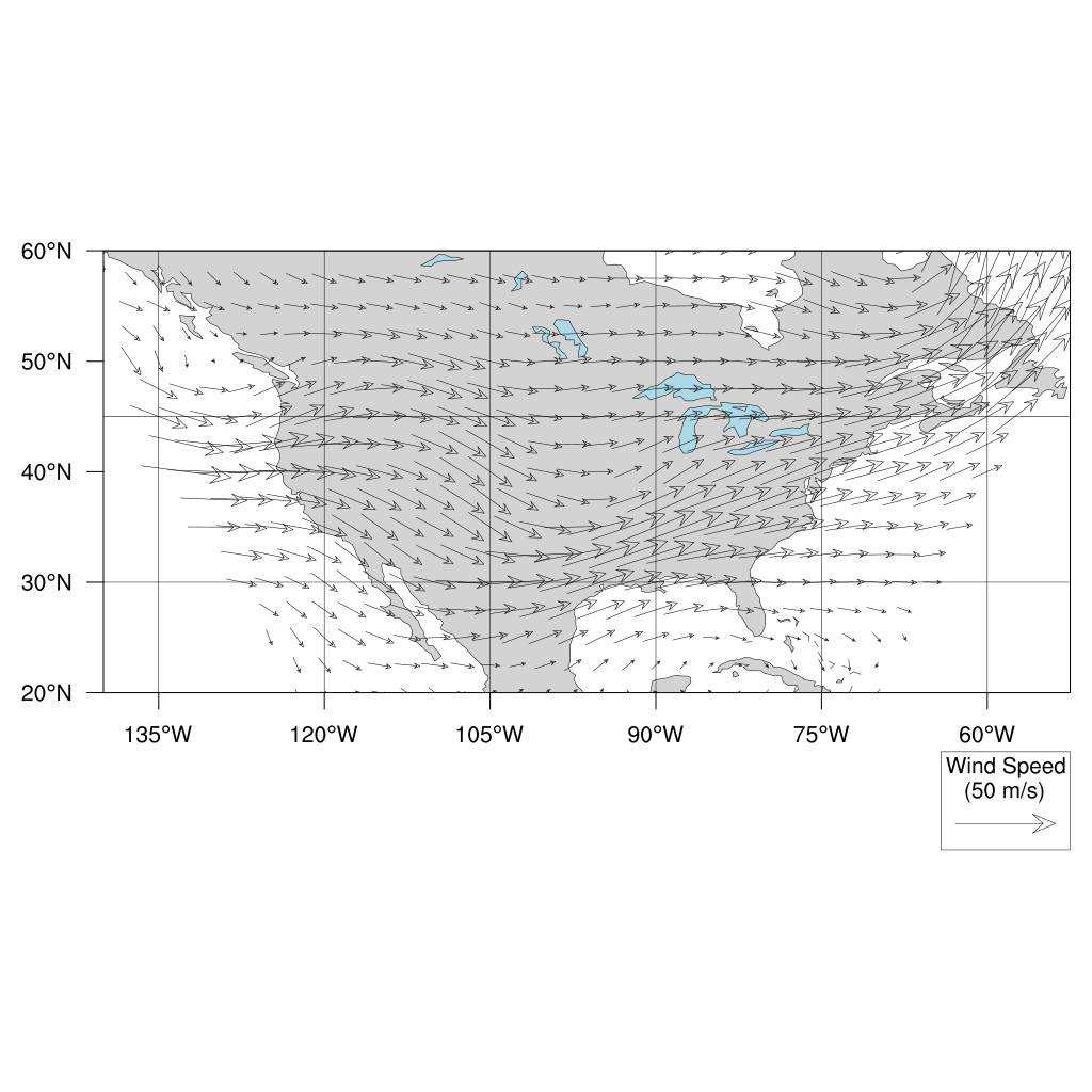
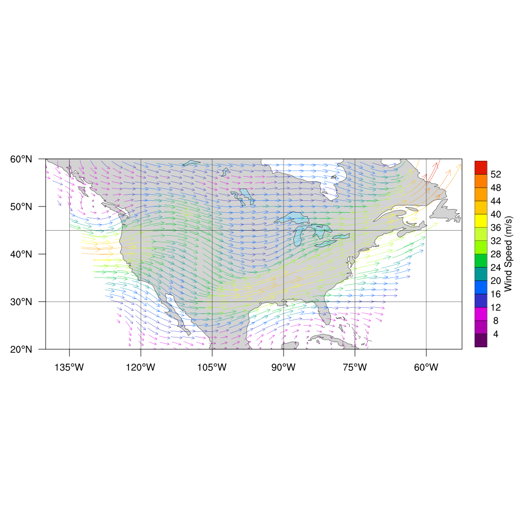
Quivers
Quivers with key
# init documents colormap
resngl = Ngl.Resources()
resngl.wkColorMap = 'precip2_15lev'
Ngl.set_values(wks, resngl)

# init plot resources
res = Ngl.Resources()

# not necessary, just a good habit
res.nglDraw = False
res.nglFrame = False

# Set map resources.
res.mpLimitMode = "LatLon"     # limit map via lat/lon
res.mpMinLatF = lat.min()         # map area
res.mpMaxLatF = lat.max()         # latitudes
res.mpMinLonF = lon.min()         # and
res.mpMaxLonF = lon.max()         # longitudes
res.mpFillOn = True
res.mpLandFillColor = "LightGray"
res.mpOceanFillColor = -1
res.mpInlandWaterFillColor = "LightBlue"

res.nglSpreadColors = True
res.nglSpreadColorEnd = 17 # index of first color for contourf
res.nglSpreadColorStart = 3 # index of last color for contourf

# coord arrays for vector plots
res.vfXArray = lon
res.vfYArray = lat

# set the annotation string. ~C~ is line break
res.vcRefAnnoString1 = "Wind Speed~C~   (50 m/s)"
res.vcRefAnnoArrowSpaceF = 0.65 # reduces white space
res.vcRefAnnoString2On = False # remove the string "Reference vector"
res.vcRefMagnitudeF  = 50.0 # speed of the reference arrow
res.vcRefLengthF     = 0.08 # length of the reference arrow
res.vcMinDistanceF = 0.02 # min. dist. between arrows

# draw the contour maps
vc = Ngl.vector_map(wks, u, v, res) # Draw a vector plot of

# draws the map
Ngl.draw(vc)

# add a page to the pdf output
Ngl.frame(wks)
Quivers with colors
res = Ngl.Resources()

# not necessary, just a good habit
res.nglDraw = False
res.nglFrame = False

# Set map resources.
res.mpLimitMode = "LatLon"     # limit map via lat/lon
res.mpMinLatF = lat.min()         # map area
res.mpMaxLatF = lat.max()         # latitudes
res.mpMinLonF = lon.min()         # and
res.mpMaxLonF = lon.max()         # longitudes
res.mpFillOn = True
res.mpLandFillColor = "LightGray"
res.mpOceanFillColor = -1
res.mpInlandWaterFillColor = "LightBlue"

# settings for the colorbar
res.lbOrientation = "Vertical" # vertical colorbar
res.lbTitleString = "Wind Speed (m/s)" # cbar title string

# the last three resources are to put the title in the right
# position for vertical cbar
res.lbTitlePosition = "Right" # cbar title position
res.lbTitleAngleF = 90
res.lbTitleDirection = "Across"

res.pmLabelBarWidthF = 0.06 # cbar width
res.lbTitleFontHeightF = 0.01
res.lbLabelFontHeightF = 0.01

res.vfXArray = lon
res.vfYArray = lat

res.nglSpreadColorEnd = 17 # index of first color for contourf
res.nglSpreadColorStart = 3 # index of last color for contourf

res.vcRefMagnitudeF  = 50.0
res.vcRefLengthF     = 0.08
res.vcMinDistanceF = 0.00
res.vcGlyphStyle = 'CurlyVector'
res.vcMonoLineArrowColor  = False   # Draw vectors in colors
res.vcRefAnnoOn = False # no reference arrow

# draw the contour maps
vc = Ngl.vector_map(wks, u, v, res) # Draw a vector plot of

# draws the map
Ngl.draw(vc)

# add a page to the pdf output
Ngl.frame(wks)

# add the colormap to see the colors
# Ngl.draw_colormap(wks)

# Ngl.end()
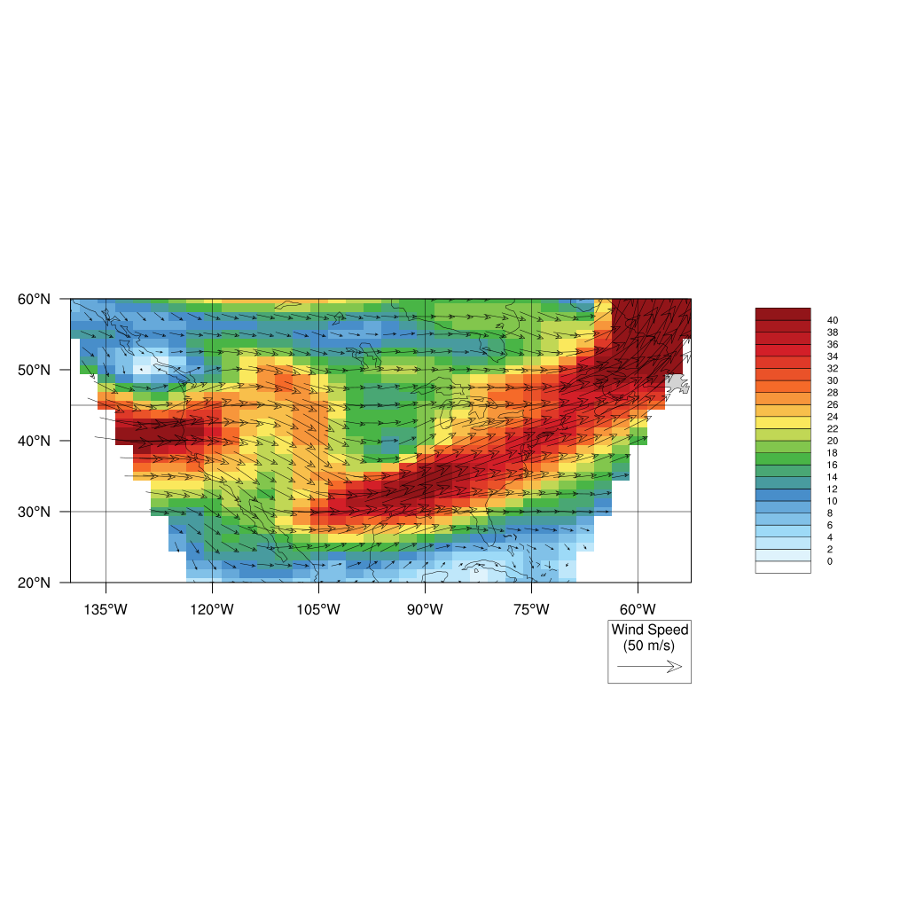
Overlays
Overlays are achived by using the Ngl.overlay method, which takes as argument the workspace and two Ngl objects (the second object is put over the first one).
# set the document colormap
resngl = Ngl.Resources()
resngl.wkColorMap = 'WhiteBlueGreenYellowRed'
Ngl.set_values(wks, resngl)

################################## Create the map contour plot
# init the plot resources
res = Ngl.Resources()

# not necessary, just a good habit
res.nglDraw = False
res.nglFrame = False

# Set map resources.
res.mpLimitMode = "LatLon"     # limit map via lat/lon
res.mpMinLatF = lat.min()         # map area
res.mpMaxLatF = lat.max()         # latitudes
res.mpMinLonF = lon.min()         # and
res.mpMaxLonF = lon.max()         # longitudes
res.mpFillOn = True
res.mpLandFillColor = "LightGray"
res.mpOceanFillColor = -1
res.mpInlandWaterFillColor = "LightBlue"

# coordinates for contour plots
res.sfXArray = lon
res.sfYArray = lat

# Set properties for contour lones
res.cnFillOn             = True # no filled contour
res.cnLinesOn            = False # contour lines
res.cnLineLabelsOn = False
res.cnInfoLabelsOn = False # add the contour info
res.cnLineThicknessF =   4 # contour lines thickness
res.cnLevelSelectionMode = "ExplicitLevels" # plotted levels are set explicitely
res.cnFillMode = "CellFill"
res.cnLevels      = np.linspace(0, 40, 21) # levels to plot

res.nglSpreadColors = True
res.nglSpreadColorStart = 2
res.nglSpreadColorEnd = 255

# draw the contour maps
m = Ngl.contour_map(wks, speed, res)

################################## Create the vector plot
resv = Ngl.Resources()

resv.gsnDraw = False
resv.gsnFrame = False

# coord arrays for vector plots
resv.vfXArray = lon
resv.vfYArray = lat

# set the annotation string. ~C~ is line break
resv.vcRefAnnoString1 = "Wind Speed~C~   (50 m/s)"
resv.vcRefAnnoArrowSpaceF = 0.65 # reduces white space
resv.vcRefAnnoString2On = False # remove the string "Reference vector"
resv.vcRefMagnitudeF  = 50.0 # speed of the reference arrow
resv.vcRefLengthF     = 0.08 # length of the reference arrow
resv.vcMinDistanceF = 0.02 # min. dist. between arrows

# Draw a vector plot. Note that here, the vector_map method is not used,
# since map projection will be managed
vplot = Ngl.vector(wks, u, v, resv)

Ngl.overlay(m, vplot)

# draws the map
Ngl.draw(m)

# add a page to the pdf output
Ngl.frame(wks)

# add the colormap to see the colors
# Ngl.draw_colormap(wks)

# Ngl.end()
warning:cnInfoLabelsOn is not a valid resource in contour at this time
warning:gsnDraw is not a valid resource in vector at this time
warning:gsnFrame is not a valid resource in vector at this time
# Finish the plot
Ngl.end()